Profiling

Summary

Supported programming model
Name	MPI	OpenMP	Cuda	SIMD
Advisor		✓		✓
Allinea MAP	✓	✓	✓	✓
Cube	✓	✓	✓	✓
Darshan	✓	✓
Gprof
cProfile
HPCToolkit	✓	✓
Igprof
IPM	✓
SelFIe
Paraver	✓	✓	✓
PAPI				✓
Perf				✓
ScoreP	✓	✓	✓
Tau	✓	✓	✓
Valgrind (cachegrind)	✓	✓
Valgrind (callgrind)	✓	✓
Valgrind (massif)	✓	✓
Vampir	✓	✓	✓
Vtune		✓		✓

Collectible events
Name	Comm	I/O	Call graph	Hardware counters	Memory usage	Cache usage
Advisor			✓
Allinea MAP	✓	✓			✓
Cube	✓	✓			✓
Darshan		✓
Gprof			✓
cProfile			✓
HPCToolkit		✓	✓	✓
Igprof					✓
IPM	✓			✓
SelFIe	✓	✓	✓			✓
Paraver	✓			✓
PAPI				✓	✓	✓
Perf		✓	✓	✓	✓	✓
ScoreP	✓		✓	✓	✓	✓
Tau	✓	✓	✓		✓
Valgrind (cachegrind)						✓
Valgrind (callgrind)			✓
Valgrind (massif)					✓
Vampir	✓
Vtune				✓		✓

Tool support and type of profiling
Name	Collection	GUI	Sampling	Tracing	Instrumentation necessary
Advisor	✓	✓	✓
Allinea MAP	✓	✓	✓	✓
Cube	✓	✓	✓	✓
Darshan	✓		✓
Gprof	✓		✓	✓	✓
cProfile	✓		✓	✓	✓
HPCToolkit	✓	✓	✓	✓
Igprof	✓		✓	✓
IPM	✓		✓
SelFIe	✓		✓
Paraver		✓		✓	✓
PAPI	✓		✓		✓
Perf			✓
ScoreP	✓		✓	✓	✓
Tau	✓	✓	✓	✓
Valgrind (cachegrind)	✓		✓
Valgrind (callgrind)	✓		✓
Valgrind (massif)	✓		✓
Vampir		✓		✓	✓
Vtune	✓	✓	✓

To display a list of all available profilers use the search option of the module command :

$ module search profiler

SelFIe

SelFIe (SElf and Light proFIling Engine) is a tool to lightly profile Linux commands without compiling. The profiling is done by a dynamic library which can be given to the LD_PRELOAD environment variable before the execution of the command. It doesn’t affect the behaviour of the command and users don’t see any changes at execution. At the end of the execution, it puts a line in system logs:

Note

SelFIe is a opensource software developed by CEA - Selfie on Github

selfie[26058]: { "utime": 0.00, "stime": 0.01, "maxmem": 0.00, "posixio_time": 0.00, "posixio_count": 7569, "USER": "user", "wtime": 0.01, "command": "/bin/hostname" }

To enable selfie:

$ module load feature/selfie/enable

To disable selfie:

$ module load feature/selfie/disable

To display the log in standard output:

$ module load feature/selfie/report

If your process takes less than 5 minutes, then load:

$ module load feature/selfie/short_job

SelFIe data can be written in a custom file by exporting the environment variable SELFIE_OUTPUTFILE:

$ export SELFIE_OUTPUTFILE=selfie.data
$ ccc_mprun -p |default_CPU_partition| -Q test -T 300 ./a.out
$ cat selfie.data
selfie[2152192]: { "utime": 0.00, "stime": 0.00, "maxmem": 0.01, "hostname": "host1216", "posixio_time": 0.00, "posixio_count": 4, "mpi_time": 0.00, "mpi_count": 0, "mpiio_time": 0.00, "mpiio_count": 0, "USER": "username", "SLURM_JOBID": "3492220", "SLURM_STEPID": "0", "SLURM_PROCID": "0", "OMP_NUM_THREADS": "1", "timestamp": 1687937047, "wtime": 30.00, "command": "./a.out" }

Example of a short job in standard output:

$ module load feature/selfie/enable
$ module load feature/selfie/report
$ module load feature/selfie/short_job
$ ccc_mprun -p |default_CPU_partition| -Q test -T 300 ./a.out

selfie[2152192]: { "utime": 0.00, "stime": 0.00, "maxmem": 0.01, "hostname": "host1216", "posixio_time": 0.00, "posixio_count": 4, "mpi_time": 0.00, "mpi_count": 0, "mpiio_time": 0.00, "mpiio_count": 0, "USER": "username", "SLURM_JOBID": "3492220", "SLURM_STEPID": "0", "SLURM_PROCID": "0", "OMP_NUM_THREADS": "1", "timestamp": 1687937047, "wtime": 30.00, "command": "./a.out" }

You can format the JSON output via the jq command:

  $ jq . <<< '{ "utime": 0.00, "stime": 0.00, "maxmem": 0.01, "hostname": "host1216", "posixio_time": 0.00, "posixio_count": 4, "mpi_time": 0.00, "mpi_count": 0, "mpiio_time": 0.00, "mpiio_count": 0, "USER": "username", "SLURM_JOBID": "3492220", "SLURM_STEPID": "0", "SLURM_PROCID": "0", "OMP_NUM_THREADS": "1", "timestamp": 1687937047, "wtime": 30.00, "command": "./a.out" }'

{
  "utime": 0,
  "stime": 0,
  "maxmem": 0.01,
  "hostname": "host1216",
  "posixio_time": 0,
  "posixio_count": 4,
  "mpi_time": 0,
  "mpi_count": 0,
  "mpiio_time": 0,
  "mpiio_count": 0,
  "USER": "username",
  "SLURM_JOBID": "3492220",
  "SLURM_STEPID": "0",
  "SLURM_PROCID": "0",
  "OMP_NUM_THREADS": "1",
  "timestamp": 1687937047,
  "wtime": 30,
  "command": "./a.out"
}

IPM

IPM is a light-weight profiling tool that profiles the mpi calls and memory usage in a parallel program. IPM cannot be used on a multi-threaded program.

To run a program with IPM profiling, just load the ipm module (no need to instrument or recompile anything) and run it with :

#!/bin/bash
#MSUB -r MyJob_Para                # Job name
#MSUB -n 32                        # Number of tasks to use
#MSUB -T 1800                      # Elapsed time limit in seconds
#MSUB -o example_%I.o              # Standard output. %I is the job id
#MSUB -e example_%I.e              # Error output. %I is the job id
#MSUB -q <partition>               # Partition name
#MSUB -A <project>                 # Project ID

set -x
cd ${BRIDGE_MSUB_PWD}

module load ipm

#The ipm module tells ccc_mprun to use IPM library
ccc_mprun ./prog.exe

It will generate a report at the end of the standard output of the job and an xml file. It is possible to generate a graphical and complete html page with the command:

$ ipm_parse -html XML_File

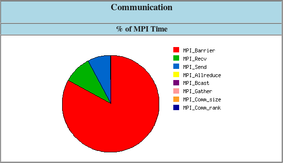
Example of IPM output

Arm-forge MAP

Arm-forge MAP is the profiler for parallel, multithreaded or single threaded C, C++ and F90 codes. MAP gives information on memory usage, MPI and OpenMP usage, percentage of vectorized SIMD instructions, etc.

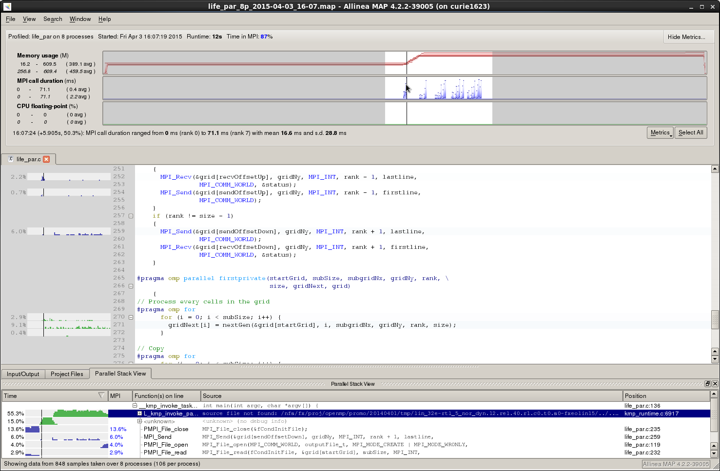
Example of MAP profile

The code just has to be compiled with -g for debugging information. No instrumentation is needed.

You can profile your code with map by loading the appropriate module:

$ module load arm-forge

Then use the command map --profile. For parallel codes, edit your submission script and just replace ccc_mprun with map --profile.

Example of submission script:

#!/bin/bash
#MSUB -r MyJob_Para                # Job name
#MSUB -q partition                 # Partition name
#MSUB -n 32                        # Number of tasks to use
#MSUB -T 1800                      # Elapsed time limit in seconds
#MSUB -o example_%I.o              # Standard output. %I is the job id
#MSUB -e example_%I.e              # Error output. %I is the job id
#MSUB -A <project>                 # Project ID
set -x
cd ${BRIDGE_MSUB_PWD}

module load arm-forge
map -n 32 ./a.out

Once the job has finished, a .map file should have been created. It can be opened from a remote desktop session or from an interactive session with the following command:

$ map <output_name>.map

Note

Arm-forge MAP is a licenced product.

Check the output of module show arm-forge or module help arm-forge to get more information on the amount of licences available.

A full documentation is available in the installation path on the cluster. To open it:

$ evince ${MAP_ROOT}/doc/userguide-forge.pdf

Scalasca

Scalasca is a set of software which let you profile your parallel code by taking traces during the execution of the program. It is actually a wrapper that launches Score-P and Cube. This software is a kind of parallel gprof with more information. We present here an introduction of Scalasca. The generated output can then be opened with several analysis tools like Periscope, Cube, Vampir, or Tau.

Scalasca profiling requires 3 different steps:

Instrumenting the code with skin
Collecting profiling data with scan
Examine collected information with square

Code instrumentation with Scalasca

First step for profiling a code with is instrumentation. You must compile your code by adding the wrapper before the call to the compiler. You need to load the scalasca module beforehand :

$ module load scalasca
$ skin mpicc -g -c prog.c
$ skin mpicc -o prog.exe prog.o

or for Fortran :

$ module load scalasca
$ skin mpif90 -g -c prog.f90
$ skin mpif90 -o prog.exe prog.o

You can compile for OpenMP programs:

$ skin ifort -openmp -g -c prog.f90
$ skin ifort -openmp -o prog.exe prog.o

You can profile hybrid MPI-OpenMP programs:

$ skin mpif90 -openmp -g -O3 -c prog.f90
$ skin mpif90 -openmp -g -O3 -o prog.exe prog.o

Simple profiling with Scalasca

Once the code has been instrumented with Scalasca, run it with scan. By default, a simple summary profile is generated.

Here is a simple example of a submission script:

#!/bin/bash
#MSUB -r MyJob_Para       # Job name
#MSUB -n 32               # Number of tasks to use
#MSUB -T 1800             # Elapsed time limit in seconds
#MSUB -o example_%I.o     # Standard output. %I is the job id
#MSUB -e example_%I.e     # Error output. %I is the job id
#MSUB -q <partition>      # Partition name
#MSUB -A <project>        # Project ID

set -x
cd ${BRIDGE_MSUB_PWD}

module load scalasca
export SCOREP_EXPERIMENT_DIRECTORY=scorep_profile.${BRIDGE_MSUB_JOBID}
scan ccc_mprun ./prog.exe

At the end of execution, the program generates a directory which contains the profiling files (the directory name is chosen with the SCOREP_EXPERIMENT_DIRECTORY environment variable):

$ tree scorep_profile.2871901
   |- profile.cubex
   `- scorep.cfg

The profile information can then be visualized with square:

$ module load scalasca
$ square scorep_profile.2871901

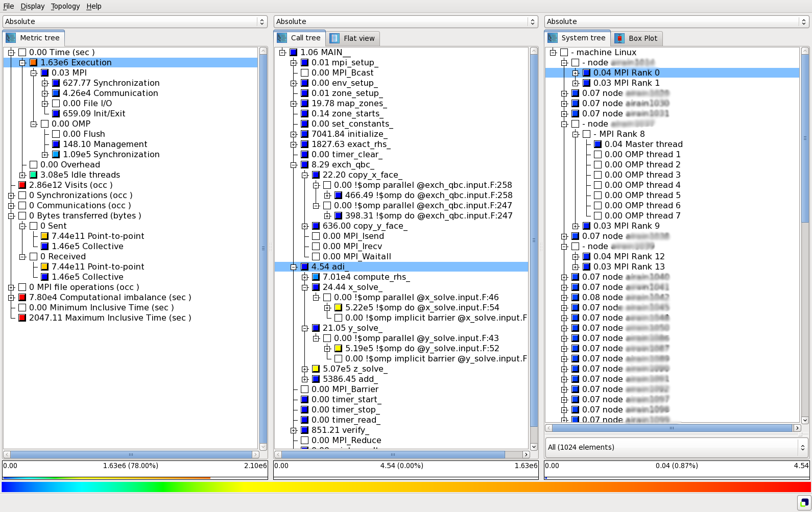
Cube interface

Scalasca with PAPI

Score-P can retrieve the hardware counter with PAPI. For example, if you want retrieve the number of floating point operations:

#!/bin/bash
#MSUB -r MyJob_Para       # Job name
#MSUB -n 32               # Number of tasks to use
#MSUB -T 1800             # Elapsed time limit in seconds
#MSUB -o example_%I.o     # Standard output. %I is the job id
#MSUB -e example_%I.e     # Error output. %I is the job id
#MSUB -q <partition>      # Partition name
#MSUB -A <project>        # Project ID

set -x
cd ${BRIDGE_MSUB_PWD}

module load scalasca
export SCOREP_EXPERIMENT_DIRECTORY=scorep_profile.${BRIDGE_MSUB_JOBID}

export SCOREP_METRIC_PAPI=PAPI_FP_OPS
scan ccc_mprun ./prog.exe

Then the number of floating point operations will appear on the profile when you visualize it. The the syntax to use several papi counters is:

export SCOREP_METRIC_PAPI="PAPI_FP_OPS,PAPI_TOT_CYC"

Tracing application with Scalasca

To get a full trace there is no need to recompile the code. The same instrumentation is used for summary and trace profiling. To activate the trace collection, use the option -t of scan.

#!/bin/bash
#MSUB -r MyJob_Para       # Job name
#MSUB -n 32               # Number of tasks to use
#MSUB -T 1800             # Elapsed time limit in seconds
#MSUB -o example_%I.o     # Standard output. %I is the job id
#MSUB -e example_%I.e     # Error output. %I is the job id
#MSUB -q <partition>      # partition name
#MSUB -A <project>        # Project ID

set -x
cd ${BRIDGE_MSUB_PWD}

module load scalasca
export SCOREP_EXPERIMENT_DIRECTORY=scorep_profile.${BRIDGE_MSUB_JOBID}
scan -t ccc_mprun ./prog.exe

In that case, a file traces.otf2 is created in the output directory with the summary. This profile trace can be opened with for example.

$ tree -L 1 scorep_profile.2727202
  |-- profile.cubex
  |-- scorep.cfg
  |-- traces/
  |-- traces.def
  `-- traces.otf2

Warning

Generating a full trace may require a huge amount of memory.

Here is the best practice to follow:

First start with a simple Scalasca analysis (without -t)
Thanks to this summary, you can get an estimation of the size a full trace would take with the command:

$ square -s scorep_profile.2871901

Estimated aggregate size of event trace:                   58GB
Estimated requirements for largest trace buffer (max_buf): 6GB
....

If the estimated aggregated size of event trace seems excessive (it can easily reach several TB), you will need to apply filtering before recording the trace.

For more information on filtering and profiling options, check out the full documentation provided in the installation path:

$ module load scalasca
$ evince ${SCALASCA_ROOT}/share/doc/scalasca/manual/UserGuide.pdf

Vampir

Vampir is a visualization software that can be used to analyse OTF traces. The traces should have been generated before by one of the available profiling software such as Score-P.

Usage

To open a Score-P trace with vampir, just launch the graphical interface with the corresponding OTF file.

$ module load vampir
$ vampir scorep_profile.2871915/traces.otf2

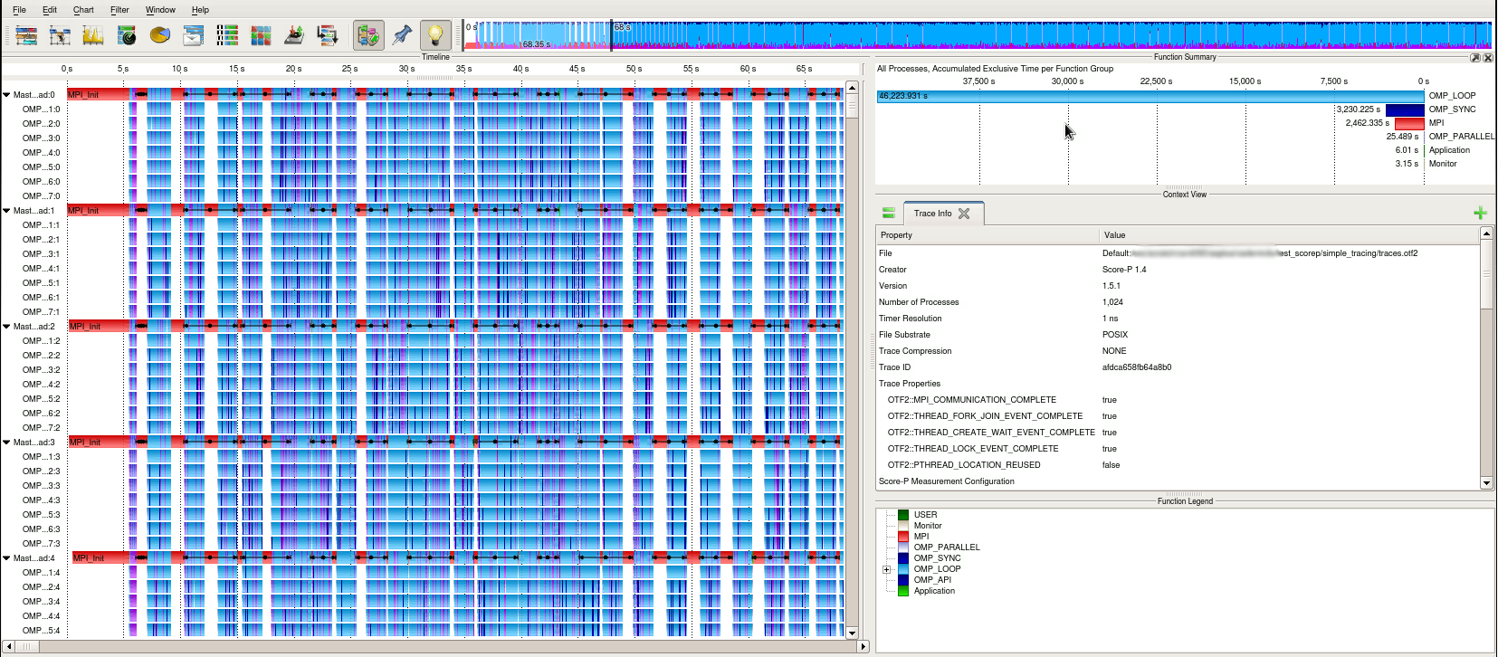
Vampir window

It is not recommended to launch on the login nodes. An interactive session on compute nodes may be necessary. Also, the graphical interface may be slow. Using the Remote Desktop System service can help with that.

See the manual for full details and features of the vampir tool.

Vampirserver

Traces generated by Score-P can be very large and can be very slow if you want to visualize these traces. Vampir provides vampirserver: it is a parallel program which uses CPU computing to accelerate Vampir visualization. Firstly, you have to submit a job which will launch on Irene nodes:

$ cat vampirserver.sh
#!/bin/bash
#MSUB -r vampirserver             # Job name
#MSUB -n 32                       # Number of tasks to use
#MSUB -T 1800                     # Elapsed time limit in seconds
#MSUB -o vampirserver_%I.o        # Standard output. %I is the job id
#MSUB -e vampirserver_%I.e        # Error output. %I is the job id
#MSUB -q partition                # Partition
#MSUB -A <project>                # Project ID


module load vampirserver
vampirserver start -n $((BRIDGE_MSUB_NPROC-1))
sleep 1700

$ ccc_msub vampirserver.sh

When the job is running, you will obtain this output:

$ ccc_mpp
USER ACCOUNT BATCHID NCPU QUEUE PRIORITY STATE RLIM  RUN/START SUSP OLD  NAME         NODES
toto genXXX  234481  32   large 210332   RUN   30.0m 1.3m      -    1.3m vampirserver node1352

$ ccc_mpeek 234481
Found license file: /usr/local/vampir-7.5/bin/lic.dat
Running 31 analysis processes... (abort with Ctrl-C or vngd-shutdown)
Server listens on: node1352:30000

And a Vampir window should open.

Note

The vampirserver command runs in the background. So, without the call to Vampir, the job would be terminated immediately.

In our example, the Vampirserver master node is on node1352. The port to connect is 30000. Now you can use the graphical interface: start Vampir on a remote desktop service. Instead of clicking on “Open”, you will click on “Remote Open”:

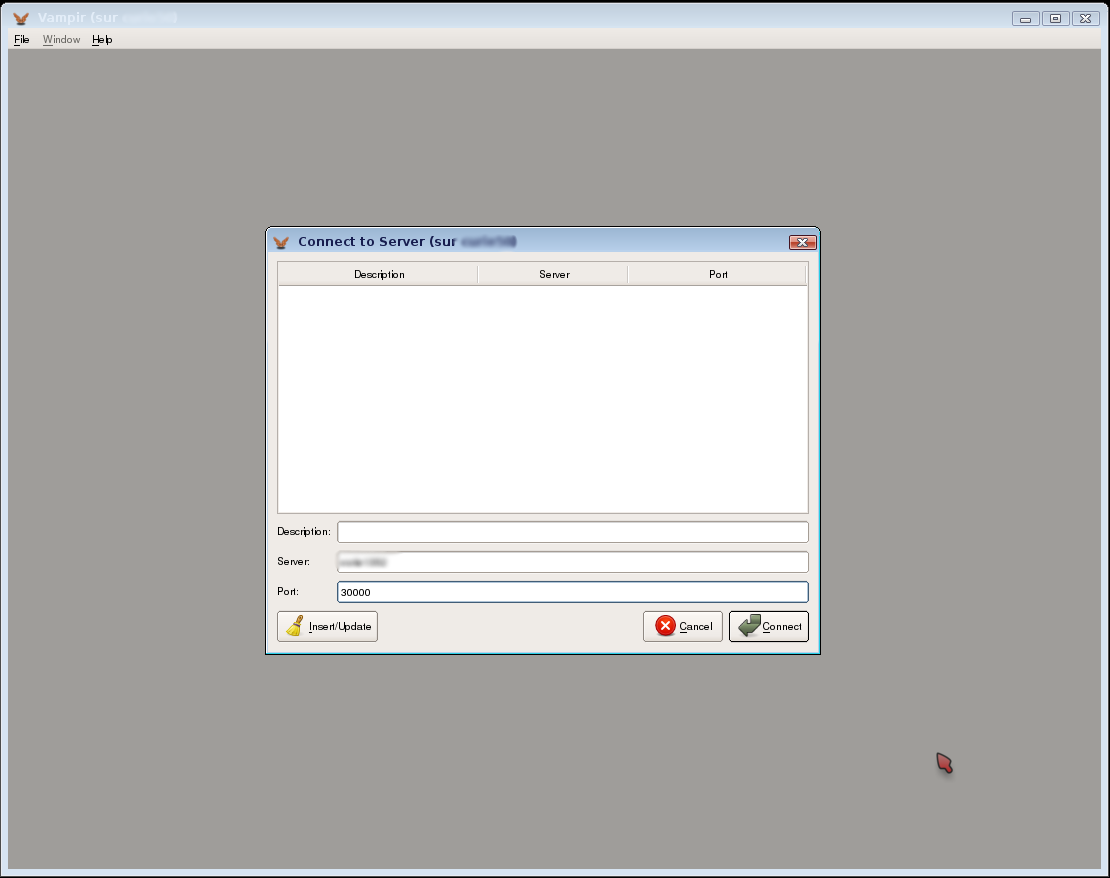
Connecting to Vampirserver

Fill the server and the port, for instance Server : node1352 and Port : 30000 in the previous case. You will be connected to vampirserver. Then you can open an OTF file and visualize it.

Note

You can ask any number of processors you want: it will be faster if your profiling files are big. But be careful, it consumes your computing times.
Don’t forget to delete the Vampirserver job after your analyse.

Score-P

Score-P is a software system that provides measurement infrastructure for profiling, event trace recording, and analysis of HPC applications. Its goal is to simplify the analysis of the behavior of HPC software and to allow developers to find out where and why performance problems arise, where bottlenecks may be expected and where their codes offer room for further improvements. Score-P supports MPI, OpenMP, Pthreads, and CUDA, OpenCL and OpenACC and Fortran, C and C++ languages. It can take traces (OTF2) to be read by Vampir or Scalasca, and call-path profiles to be read by CUBE or TAU.

Instrumentation

Score-P is available through the module command:

$ module load scorep

You need to compile your code with scorep. Compile and link with:

scorep mpicc for C code source files,
scorep mpicxx for C++ code source files, and
scorep mpif90 for Fortran code source files,

Usage

The command to run scorep is:

$ ccc_mprun -n $NPROCS  ./my_app

When running the instrumented exectuable, the measurement system will create a directory called scorep-YYYYMMDD_HHMM_XXXXXXX, containing the date and time, and where XXXXXXXX is an additional identification number. The environment variables SCOREP_ENABLE_TRACING and SCOREP_ENABLE_PROFILING control whether event tracing or profiles are stored in this directory. By default, profiling is enabled and tracing is disabled.

After the completion of the execution, the requested data is available in the dedicated location, and can be visualized and analized by CUBE, TAU, or Vampir, for example.

For more information, see Score-P User Guide.

Darshan

Darshan is a scalable HPC I/O characterization tool. It is designed to profile I/O behavior with minimum overhead.

To run a program with Darshan profiling, there is no need to instrument or recompile the code.

Load the darshan module : it tells ccc_mprun to wrap the I/O calls with the Darshan library.
Specify where you want the darshan trace to be created by exporting the variable DARSHAN_LOG_PATH.

Here is an example of a submission script to enable darshan profiling:

#!/bin/bas
#MSUB -r MyJob_Para       # Job name
#MSUB -n 32               # Number of tasks to use
#MSUB -T 1800             # Elapsed time limit in seconds
#MSUB -o example_%I.o     # Standard output. %I is the job id
#MSUB -e example_%I.e     # Error output. %I is the job id
#MSUB -q <partition>      # Partition
#MSUB -A <project>        # Project ID

set -x
cd ${BRIDGE_MSUB_PWD}

module load darshan
export DARSHAN_LOG_PATH=$PWD

#The darshan module tells ccc_mprun to use the Darshan library.
ccc_mprun ./prog.exe

This will generate a trace in the specified directory. Here is the format of the output file: <USERNAME>_<BINARY_NAME>_<JOB_ID>_<DATE>_<UNIQUE_ID>_<TIMING>.darshan.gz.

Some scripts are available to post-process the output. For instance, darshan-parser, darshan-job-summary.pl and darshan-summary-per-file.sh.

darshan-job-summary.pl will generate a graphical summary of the I/O activity for a job.

$ darshan-job-summary.pl *.darshan.gz

darshan-summary-per-file.sh is similar except that it produces a separate pdf summary for every file accessed by the application. The summaries will be written in the directory specified as argument.

$ darshan-summary-per-file.sh *.darshan.gz output_dir

darshan-parser gives a full, human readable dump of all information contained in a log file.

$ darshan-parser *.darshan.gz > example_output.txt

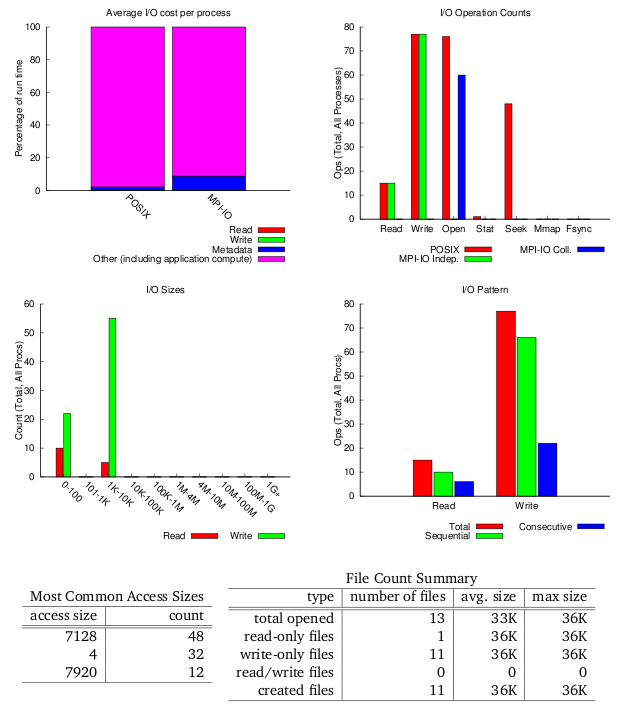
Example of Darshan output

PAPI

PAPI is an API which allows you to retrieve hardware counters from the CPU. Here an example in Fortran to get the number of floating point operations of a matrix DAXPY:

program main
 implicit none
 include 'f90papi.h'
 !
 integer, parameter :: size = 1000
 integer, parameter :: ntimes = 10
 double precision, dimension(size,size) :: A,B,C
 integer :: i,j,n
 ! Variable PAPI
 integer, parameter :: max_event = 1
 integer, dimension(max_event) :: event
 integer :: num_events, retval
 integer(kind=8), dimension(max_event) :: values
 ! Init PAPI
 call PAPIf_num_counters( num_events )
 print *, 'Number of hardware counters supported: ', num_events
 call PAPIf_query_event(PAPI_FP_INS, retval)
 if (retval .NE. PAPI_OK) then
    event(1) = PAPI_TOT_INS
 else
    ! Total floating point operations
    event(1) = PAPI_FP_INS
 end if
 ! Init Matrix
 do i=1,size
    do j=1,size
       C(i,j) = real(i+j,8)
       B(i,j) = -i+0.1*j
    end do
 end do
 ! Set up counters
 num_events = 1
 call PAPIf_start_counters( event, num_events, retval)
 ! Clear the counter values
 call PAPIf_read_counters(values, num_events,retval)
 ! DAXPY
 do n=1,ntimes
    do i=1,size
       do j=1,size
          A(i,j) = 2.0*B(i,j) + C(i,j)
       end do
    end do
 end do
 ! Stop the counters and put the results in the array values
 call PAPIf_stop_counters(values,num_events,retval)
 ! Print results
 if (event(1) .EQ. PAPI_TOT_INS) then
    print *, 'TOT Instructions:  ',values(1)
 else
    print *, 'FP Instructions:  ',values(1)
 end if
end program main

To compile, you have to load the PAPI module:

bash-4.00 $ module load papi/4.2.1
bash-4.00 $ ifort ${PAPI_CFLAGS} papi.f90 ${PAPI_LDFLAGS}
bash-4.00 $ ./a.out
 Number of hardware counters supported:            7
 FP Instructions:                10046163

To get the available hardware counters, you can type papi_avail command.

This library can retrieve the MFLOPS of a certain region of your code:

program main
 implicit none
 include 'f90papi.h'
 !
 integer, parameter :: size = 1000
 integer, parameter :: ntimes = 100
 double precision, dimension(size,size) :: A,B,C
 integer :: i,j,n
 ! Variable PAPI
 integer :: retval
 real(kind=4) :: proc_time, mflops, real_time
 integer(kind=8) ::  flpins
 ! Init PAPI
 retval = PAPI_VER_CURRENT
 call PAPIf_library_init(retval)
 if ( retval.NE.PAPI_VER_CURRENT) then
    print*, 'PAPI_library_init', retval
 end if
 call PAPIf_query_event(PAPI_FP_INS, retval)
 ! Init Matrix
 do i=1,size
    do j=1,size
       C(i,j) = real(i+j,8)
       B(i,j) = -i+0.1*j
    end do
 end do
 ! Setup Counter
 call PAPIf_flips( real_time, proc_time, flpins, mflops, retval )
 ! DAXPY
 do n=1,ntimes
    do i=1,size
       do j=1,size
          A(i,j) = 2.0*B(i,j) + C(i,j)
       end do
    end do
 end do
 ! Collect the data into the Variables passed in
 call PAPIf_flips( real_time, proc_time, flpins, mflops, retval)
 ! Print results
 print *, 'Real_time: ', real_time
 print *, ' Proc_time: ', proc_time
 print *, ' Total flpins: ', flpins
 print *, ' MFLOPS: ', mflops
 !
end program main

and the output:

bash-4.00 $ module load papi/4.2.1
bash-4.00 $ ifort ${PAPI_CFLAGS} papi_flops.f90 ${PAPI_LDFLAGS}
bash-4.00 $ ./a.out
 Real_time:   6.1250001E-02
  Proc_time:   5.1447589E-02
  Total flpins:              100056592
  MFLOPS:    1944.826

If you want more precisions, you can contact us or visit PAPI website.

Valgrind

Valgrind is an instrumentation framework for dynamic analysis tools. It comes with a set of tools for profiling and debugging codes.

To run a program with valgrind, there is no need to instrument, recompile, or otherwise modify the code.

Note

A tool in the Valgrind distribution can be invoked with the --tool option:

module load valgrind
valgrind --tool=<toolname> #default is memcheck

Callgrind

Callgrind is a profiling tool that records the call history among functions in a program’s run as a call-graph. By default, the collected data consists of the number of instructions executed, their relationship to source lines, the caller/callee relationship between functions, and the numbers of such calls.

To start a profile run for a program, execute:

module load valgrind
valgrind --tool=callgrind [callgrind options] your-program [program options]

While the simulation is running, you can observe the execution with:

callgrind_control -b

This will print out the current backtrace. To annotate the backtrace with event counts, run:

callgrind_control -e -b

After program termination, a profile data file named callgrind.out.<pid> is generated, where pid is the process ID of the program being profiled. The data file contains information about the calls made in the program among the functions executed, together with Instruction Read (Ir) event counts.

To generate a function-by-function summary from the profile data file, use:

callgrind_annotate [options] callgrind.out.<pid>

Cachegrind

Cachegrind simulates how your program interacts with a machine’s cache hierarchy and (optionally) branch predictor. To run cachegrind on a program prog, you must specify --tool=cachegrind on the valgrind command line:

module load valgrind
valgrind --tool=cachegrind prog

Branch prediction statistics are not collected by default. To do so, add the option --branch-sim=yes.

valgrind -tool=cachegrind --branch-sim=yes prog

One output file will be created for each process launched with cachegrind. To analyse the output, use the command cg_annotate:

$ cg_annotate <output_file>

cg_annotate can show the source codes annotated with the sampled values. Therefore, either use the option --auto=yes to apply to all the available source files or specify one file by passing it as an argument.

$ cg_annotate <output_file> sourcecode.c

For more information on Cachegrind, check out the official Cachegrind User Manual.

Massif

Massif measures how much heap memory a program uses. This includes both the useful space, and the extra bytes allocated for book-keeping and alignment purposes. Massif can optionally measure the stack memory.

As for the other Valgrind tools, the program should be compiled with debugging info (the -g option). To run massif on a program prog, the valgrind command line is:

module load valgrind
valgrind --tool=massif prog

The Massif option --pages-as-heap=yes allows to measure all the memory used by the program.

By default, the output file is called massif.out.<pid> (pid is the process ID), although this file name can be changed with the --massif-out-file option. To present the heap profiling information about the program in a readable way, run ms_print:

$ ms_print massif.out.<pid>

TAU (Tuning and Analysis Utilities)

TAU Performance System is a portable profiling and tracing toolkit for performance analysis of parallel programs written in Fortran, C, C++, UPC, Java, Python.

TAU (Tuning and Analysis Utilities) is capable of gathering performance information through instrumentation of functions, methods, basic blocks, and statements as well as event-based sampling. The instrumentation can be inserted in the source code using an automatic instrumentor tool based on the Program Database Toolkit (PDT), dynamically using DyninstAPI, at runtime in the Java Virtual Machine, or manually using the instrumentation API.

TAU’s profile visualization tool, paraprof, provides graphical displays of all the performance analysis results, in aggregate and single node/context/thread forms. The user can quickly identify sources of performance bottlenecks in the application using the graphical interface. In addition, TAU can generate event traces that can be displayed with the Vampir, Paraver or JumpShot trace visualization tools.

Instrumentation

TAU is available through the module command:

$ module load tau

Specify programming model by setting TAU_MAKEFILE to one of $TAU_MAKEFILEDIR/Makefile.tau-*:

Makefile.tau-icpc-papi-mpi-cupti-pdt-openmp

Compile and link with:

tau_cc.sh for C code source files,
tau_cxx.sh for C++ code source files, and
tau_f90.sh for Fortran code source files,

Usage

The command to run TAU is:

$ ccc_mprun -n $NPROCS tau_exec ./a.out

Examine results with paraprof/pprof

$ pprof [directory_path]

or

$ paraprof

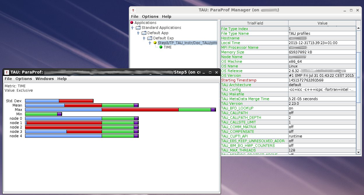
Example of ParaProf window

Note

It’s recommended to use the Remote Desktop session to use the graphical tools provided by tau (e.g. paraprof).

Environment variables control measurement mode TAU_PROFILE, TAU_TRACE, TAU_CALLPATH are available to tune the profiling settings.

For more information, see TAU User Guide.

Perf

Perf is a portable tool included in Linux kernel, it doesn’t need to be loaded, doesn’t need any driver and also works on all Linux platforms.

It is a performance analysis tool which displays performance counters such as the number of cache loads misses or branch loads misses.

Perf cannot be fully launched on login nodes, you will need to execute it on compute node(s).
In order to profile several processes with perf, you will need to differentiate the outputs by processe. Here is a simple wrapper to do it :

$ cat wrapper_perf.sh
#!/bin/bash
perf record -o out.${SLURM_PROCID}.data $@

To run a command and gather performance counter statistics use perf stat. Here is a simple job example:

#!/bin/bash
#MSUB -n 4
#MSUB -c 12
#MSUB -T 400
#MSUB -q |Partition|
#MSUB -A <project>
#MSUB -x
#MSUB -E '--enable_perf'

export OMP_NUM_THREADS=${BRIDGE_MSUB_NCORE}

ccc_mprun wrapper_perf stat ./exe

Informations will be stored in out.<jobID>.data:

$ cat out.0.data
# started on Wed Oct 11 14:01:14 2017

Performance counter stats for './exe':

  50342.076495         task-clock:u (msec)       #    1.000 CPUs utilized
  98,323               page-faults:u             #    0.002 M/sec
  155,516,791,925      cycles:u                  #    3.089 GHz
  197,715,764,466      instructions:u            #    1.27  insn per cycle

    50.348439743 seconds time elapsed

Now for more specifics counters:

list of all performance counters with the command perf list
Use the -e option to specify the wanted performance counters. For example, to get how much cache access misses within all cache access:

$ ccc_mprun perf stat -o perf.log -e cache-references,cache-misses ./exe
$ cat perf.log
# started on Wed Oct 11 14:02:52 2017

Performance counter stats for './exe':

  8,654,163,728      cache-references:u
  875,346,349        cache-misses:u            #   10.115 % of all cache refs

    52.710267128 seconds time elapsed

Perf can also record few counters from an executable and create a report:

Use a job to create a report with

$ ccc_mprun -vvv perf record -o data.perf ./exe
...
[ perf record: Woken up 53 times to write data ]
[ perf record: Captured and wrote 13.149 MB data.perf (344150 samples) ]
...

Read the report from the login node

$ perf report -i data.perf
Samples: 344K of event 'cycles:u', Event count (approx.): 245940413046
Overhead  Command  Shared Object       Symbol
 99.94%  exe      exe                 [.] mydgemm_
  0.02%  exe      [kernel.vmlinux]    [k] apic_timer_interrupt
  0.02%  exe      [kernel.vmlinux]    [k] page_fault
  0.00%  exe      exe                 [.] MAIN__
  ...

You can also using call graphs with

$ ccc_mprun -vvv perf record --call-graph fp -o data.perf ./exe

$ perf report -i data.perf
Samples: 5K of event 'cycles:u', Event count (approx.): 2184801676
 Children      Self  Command  Shared Object           Symbol
+   66.72%     0.00%  exe      libc-2.17.so            [.] __libc_start_main
+   61.03%     0.03%  exe      libiomp5.so             [.] __kmpc_fork_call
-   60.96%     0.05%  exe      libiomp5.so             [.] __kmp_fork_call
    60.90% __kmp_fork_call
     - __kmp_invoke_microtask
          56.06% nextGen
          3.33% main
          1.35% __intel_avx_rep_memcpy
+   60.90%     0.03%  exe      libiomp5.so             [.] __kmp_invoke_microtask
+   56.06%    56.06%  exe      exe                     [.] nextGen
+    8.98%     5.86%  exe      exe                     [.] main
...

Extra-P

Extra-P is an automatic performance-modeling tool that can be used to analyse several SCOREP_EXPERIMENT_DIRECTORY generated with Score-P. The primary goal of this tool is identify scalability bugs but due to his multiple graphics outputs, it’s also useful to make reports.

Usage

To analyse the scalability of an algorithm you need to generate several SCOREP_EXPERIMENT_DIRECTORY, for example you can launch this submission script:

#!/bin/bash
#MSUB -r npb_btmz_scorep
#MSUB -o npb_btmz_scorep_%I.o
#MSUB -e npb_btmz_scorep_%I.e
#MSUB -Q test
#MSUB -T 1800    # max walltime in seconds
#MSUB -q haswell
#MSUB -A <project>

cd $BRIDGE_MSUB_PWD

# benchmark configuration
export OMP_NUM_THREADS=$BRIDGE_MSUB_NCORE

# Score-P configuration
export SCOREP_EXPERIMENT_DIRECTORY=scorep_profile.p$p.r$r
PROCS=$BRIDGE_MSUB_NPROC
EXE=./exe

ccc_mprun -n $PROCS $EXE

from a bash script (4 runs on each scripts with 8, 16, 32 and 64 cores):

p=4 n=2 c=2 r=1 ccc_msub -n 2 -c 2 submit_global.msub
p=4 n=2 c=2 r=2 ccc_msub -n 2 -c 2 submit_global.msub
p=4 n=2 c=2 r=3 ccc_msub -n 2 -c 2 submit_global.msub
p=4 n=2 c=2 r=4 ccc_msub -n 2 -c 2 submit_global.msub
p=8 n=2 c=4 r=1 ccc_msub -n 2 -c 4 submit_global.msub
[...]
p=32 n=8 c=4 r=4 ccc_msub -n 8 -c 4 submit_global.msub
p=64 n=8 c=8 r=1 ccc_msub -n 8 -c 8 submit_global.msub
p=64 n=8 c=8 r=2 ccc_msub -n 8 -c 8 submit_global.msub
p=64 n=8 c=8 r=3 ccc_msub -n 8 -c 8 submit_global.msub
p=64 n=8 c=8 r=4 ccc_msub -n 8 -c 8 submit_global.msub

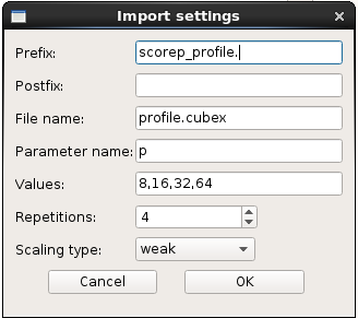
Once these folders are generated load Extra-P:

$ module load extrap

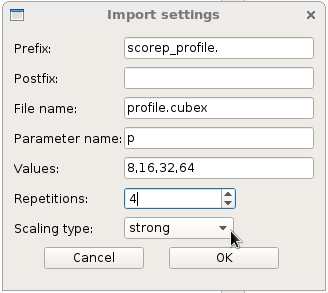
launch it and open the parent folder. The software detects automatically your files:

On Metric section choose “time” and you will get the time of each commands. You can also right clic on the graph and choose “Show all data points”, you will see the time of all your runs:

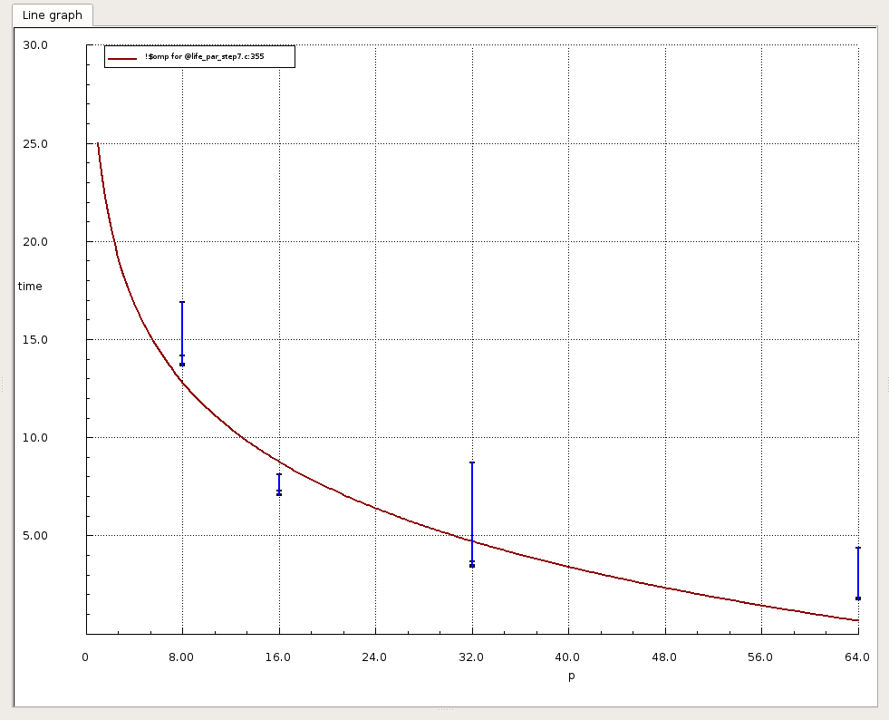
Note

These graphics only give the time of your application, not any speedup.

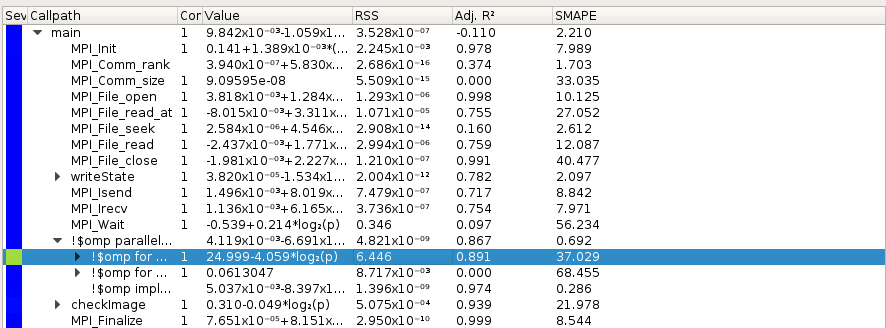
Extra-P also list all MPI and OpenMP requests, you can select what you want and check scalability:

At least, you can choose to use strong scaling and see the efficiency of an algorithm:

Gprof

Gprof produces an execution profile of C/C++ and Fortran programs. The effect of called routines is incorporated in the profile of each caller. The profile data is taken from the call graph profile file (gmon.out default) which is created by programs that are compiled with the -pg option. Gprof reads the given object file (the default is “a.out”) and establishes the relation between its symbol table and the call graph profile from gmon.out.

To load gprof:

$ module load gprof

To compile with -pg option

$ icc -pg hello.c

If your application is MPI, set environment variable to rename gmon files and enable one file per process

$ export GMON_OUT_PREFIX='gmon.out-'`/bin/uname -n`

Files generated will be named gmon.out-<hostname>.<pid> (ie: gmon.out-node1192.56893).

To generate call graph profile gmon.out

$ ./a.out

To display flat profile and call graph

$ gprof a.out gmon.out

To display only the flat profile

$ gprof -p -b ./a.out gmon.out

Flat profile:
Each sample counts as 0.01 seconds.
 %   cumulative   self              self     total
time   seconds   seconds    calls   s/call   s/call  name
67.72     10.24    10.24        1    10.24    10.24  bar
33.06     15.24     5.00                             main
 0.00     15.24     0.00        1     0.00    10.24  foo

To display the flat profile of one specific routine

$ gprof -p<routine> -b ./a.out gmon.out

To display only the call graph

$ gprof -q -b ./a.out gmon.out

Call graph (explanation follows)
index % time    self  children    called     name
                                                <spontaneous>
[1]    100.0    5.00   10.24                 main [1]
                0.00   10.24       1/1           foo [3]
-----------------------------------------------
               10.24    0.00       1/1           foo [3]
[2]     67.2   10.24    0.00       1         bar [2]
-----------------------------------------------
               0.00   10.24       1/1           main [1]
[3]     67.2   0.00   10.24        1         foo [3]
               10.24    0.00       1/1           bar [2]
-----------------------------------------------

To display the call graph of one specific routine

$ gprof -q<routine> -b ./a.out gmon.out

To generate a graph from data, see gprof2dot and gprof

Gprof2dot

Gprof2dot is an utility which converts profile data into a dot graph. It is compatible with many profilers.

Use with gprof

Load modules gprof AND gprof2dot

$ module load gprof gprof2dot

Be sure to compile your application with -pg option

$ icc -pg hello.c

Generate the call graph profile gmon.out (Run the application one time)

$ ./a.out

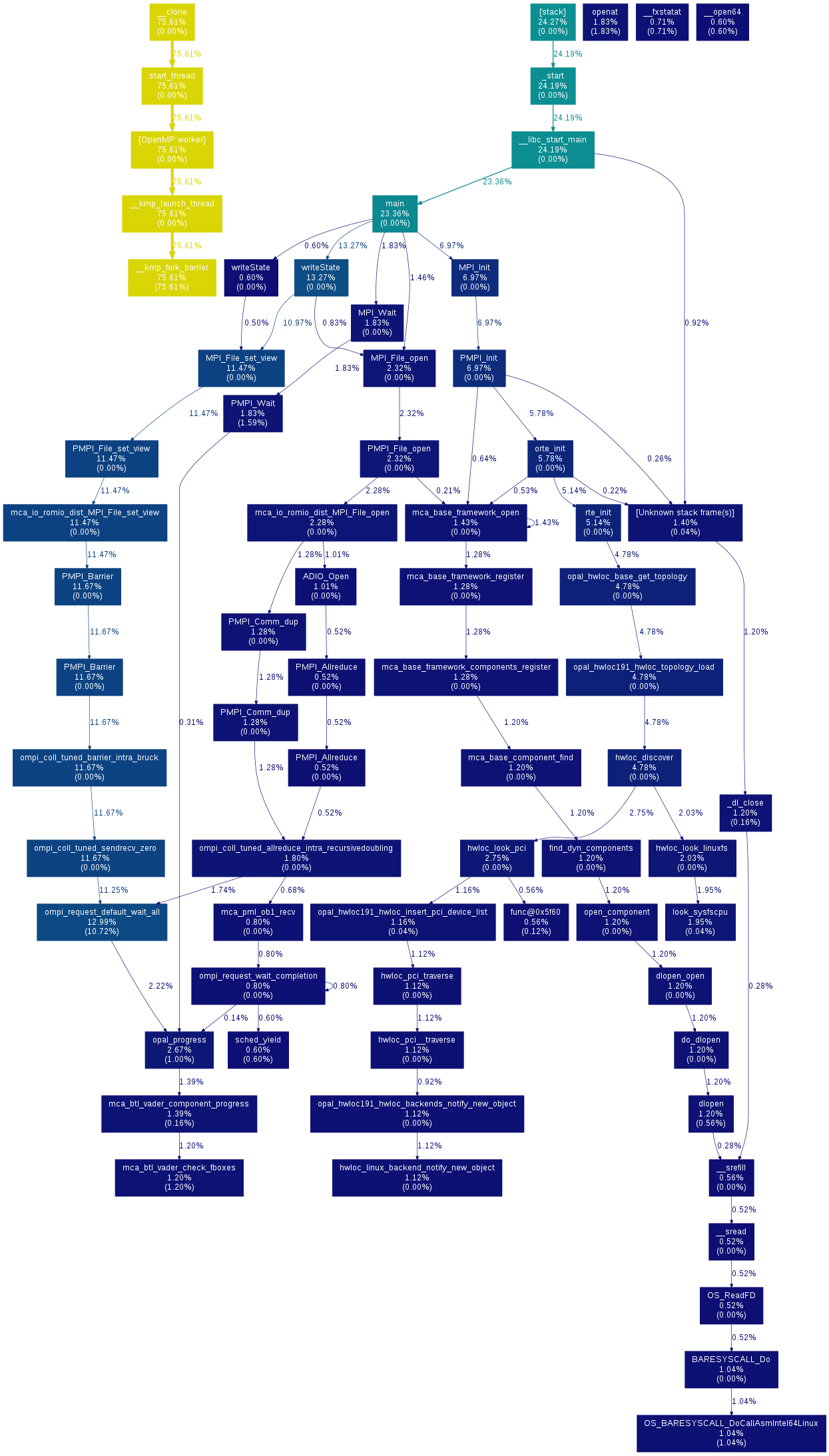
Generate the dot graph in a PNG image

$ gprof ./a.out gmon.out | gprof2dot.py | dot -Tpng -o a.png

Use with VTune in command line

Load modules VTune AND gprof2dot

$ module load vtune gprof2dot

Use VTune to collect data

$ ccc_mprun amplxe-cl -collect hotspots -result-dir output -- ./exe

Transform data in a gprof-like file

$ amplxe-cl -report gprof-cc -result-dir output -format text -report-output output.txt

Generate the dot graph

$ gprof2dot.py -f axe output.txt | dot -Tpng -o output.png

For more information about gprof2dot, see GitHub gprof2dot.

cProfile: Python profiler

cProfile is a profiler included with Python. It returns a set of statistics that describes how often and for how long various parts of the program executed.

First, load python3 module:

$ module load python3

Then, use -m cProfile option of the python3 command:

$ python3 -m cProfile monte_carlo_pi.py

Sorting by cumulative:
Estimated value of pi: 3.1413716
         40001353 function calls (40001326 primitive calls) in 17.496 seconds

    Ordered by: cumulative time

    ncalls  tottime  percall  cumtime  percall filename:lineno(function)
      3/1    0.000    0.000   17.496   17.496 {built-in method builtins.exec}
        1    0.000    0.000   17.496   17.496 monte_carlo_pi.py:1(<module>)
        1    0.000    0.000   17.489   17.489 monte_carlo_pi.py:16(main)
        1    9.232    9.232   17.489   17.489 monte_carlo_pi.py:3(estimate_pi)
 20000000    6.687    0.000    8.257    0.000 random.py:415(uniform)

The output can be ordered by several keys, use the -s option to select:

$ python3 -m cProfile -s cumulative monte_carlo_pi.py

Here is a table of acceptable keys:

Sort Key	Description
calls	Number of times the function was called
cumulative	Total time spent in the function and all the functions it calls
cumtime	Total time spent in the function and all the functions it calls
file	Filename where the function is defined
filename	Filename where the function is defined
module	Filename where the function is defined
ncalls	Number of times the function was called
pcalls	Number of primitive (i.e., not induced via recursion) function calls
line	Line number in the file where the function is defined
name	Name of the function
nfl	Combination of function name, filename, and line number
stdname	Standard function name (a more readable version of ‘nfl’)
time	Internal time spent in the function excluding time made in calls to sub-functions
tottime	Internal time spent in the function excluding time made in calls to sub-functions

Functions profiling

cProfile is a powerful tool for profiling Python scripts. However, it’s not always efficient to profile an entire script, especially if you have a specific function suspected to be a performance bottleneck.

In computational programs, a heavy-lifting function, such as one performing complex calculations or data manipulations, often consumes a significant portion of the execution time. Profiling this specific function can provide more granular insights, assisting in identifying areas for optimization.

Here’s how to use cProfile for a specific function:

import cProfile

def my_compute_func():
    # Complex computation function

cProfile.run('my_compute_func()', sort='cumulative')

Targeted profiling helps optimize the most time-consuming parts of your code, potentially resulting in substantial improvements in the overall execution time.

cProfile and mpi4py

It is possible to profile MPI code using cProfile, but it can be a bit more complex than profiling a single process Python script.

When an MPI program is run, multiple processes are created, each with its own Python interpreter. If you just run cProfile as usual, each process will attempt to write its profiling data to the same file, which will lead to problems.

To avoid this, you can modify your MPI script to write the profiling data from each process to a different file. Here is an example using mpi4py:

from mpi4py import MPI
import cProfile

def main(rank):
    # Your MPI code here
    pass

if __name__ == "__main__":
    comm = MPI.COMM_WORLD
    rank = comm.Get_rank()
    cProfile.run('main(rank)', f'output_{rank}.pstats')

Please remember that this way, the result is a number of different files each representing the profiling results of one MPI process. They won’t give you a total view of the time spent across all processes, but you will be able to see what each individual process spent its time on.

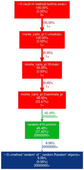
cProfile and gprof2dot

cProfile output can be formatted into reports via the pstats module:

$ python3 -m cProfile -o output.pstats monte_carlo_pi.py

The pstats file is readable by gprof2dot:

$ module load gprof2dot
$ gprof2dot.py -f pstats output.pstats -o output.dot
$ dot -Tpng output.dot -o output.png

Then, display output.png with eog or display command.

Nsight System

nsys is a profiler and graphical profile data analysis tool for CUDA applications. It is installed with the Nvidia HPC Software Development Kit and can be accessed through the nvhpc module.

In order to profile your application, you can use the following startup command in a job script :

ccc_mprun nsys profile --trace=openacc,cuda,mpi,nvtx --stats=true ./set_visible_device.sh ./myprogram`

During execution, nsys will creates report<n>.sqlite and report<n>.nsys-rep files.

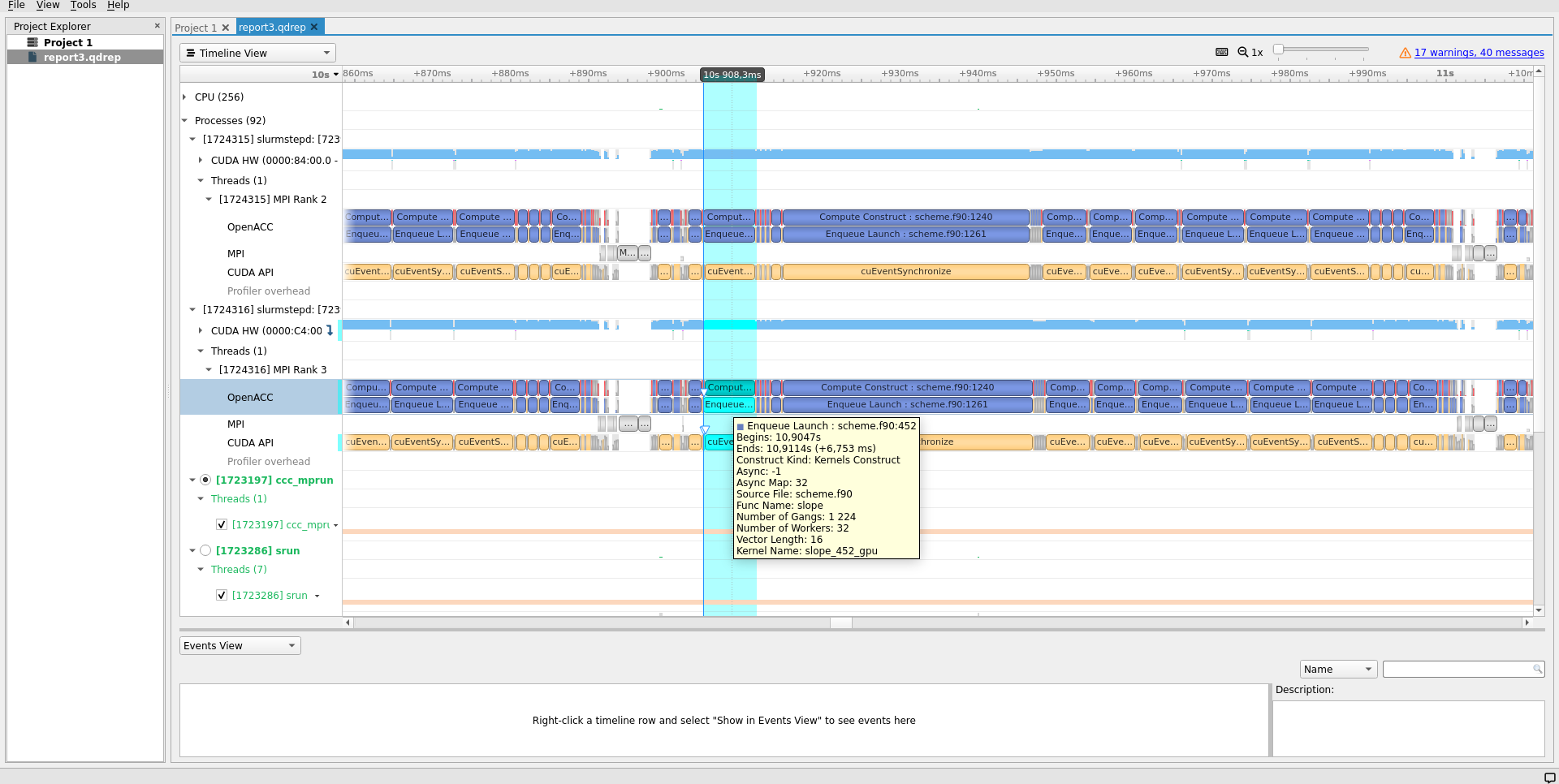
You may then use the command line or graphical interface to analyse and display these results. nsys-ui starts up the graphical interface. Use nsys-ui path/to/report*.nsys-rep to open up the nsys report files and navigate the collected traces.

../../_images/nsys-screenshot-dumses.png

For convenience, you may install Nsight Systems on your own computer and copy the instrumentation data there for displaying. Nsight Systems is freely available to members of the NVIDIA Developer Program which is a free registration. Note that you will need to select the right version for download. Use nsys --version to know which one is being used in your profiling jobs.

The nsys-ui graphical interface can also be used to launch computations directly on nodes reserved, eg. using ccc_mprun -K.

Refer to the online Nsight Systems documentation or to the nsys --help command for more information

Warning

A known bug affects nsys MPI auto-detection feature when using OpenMPI 4.1.x versions which produces a segmentation fault. In order to circumvent it, use the --mpi-impl=openmpi option.

Nsight Compute

ncu is a cuda kernel profiler for analysing GPU occupancy, and the usage of memory and compute units. It features advanced performance analysis tools and a graphical reporting interface providing useful hints and graphs.

In order to profile your application kernels, you may use the following startup command in a job script :

ccc_mprun ncu --call-stack --nvtx --set full -s 20 -c 20 --target-processes all -o report_%q{SLURM_PROCID} ./set_visible_device.sh ./myprogram

This example will generate one report file, named report_X.ncu-rep, for each process started by the application.

It uses the full argument to the --set option, which triggers the collection of a set of metrics.

You may use other values for the --set option for specifying a chosen set of sections, use --section for enabling individual report sections and the associated metrics, or use --metric for activating the collection of individual metrics. Use ncu --list-sets, ncu --list-sections and ncu --list-metrics respectively for more informations.

The option -s 20 ignores the first 20 kernels executed, in an attempt to avoid gathering information on kernels which are not representative of the general workload, such as those in charge of data initialization.

The option -c 20 enables the profiling and collection of selected performance metrics for the next 20 kernels, providing control over the general overhead of profiling the executed program.

For more information, run ncu --help or refer to the online Nsight Compute CLI documentation.

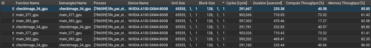
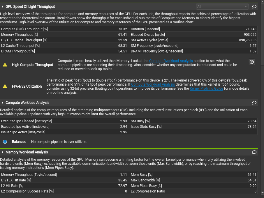
Use the ncu-ui command to open the generated reports in the Nsight Compute GUI, and access the various performance analysis, hints, and graphs.

For more information, please refer to the online Nsight Compute documentation