Quantum software stack
Quantum computing at TGCC
Quantum computing at TGCC is made available through an offer of hardware, today including emulators and simulators, and a comprehensive software stack.
This quantum service can be used to emulate quantum problems on cluster nodes or on Qaptiva emulator, and to execute quantum programs on Pasqal QPU.
On the hardware side, apart from compute nodes that can be used to emulate quantum systems, we provide a Qaptiva emulator (a dedicated hardware to quantum emulation) as well as a physical QPUs from Pasqal.
To run quantum algorithms, we provide a comprehensive software stack, notably including myQLM (with many features from digital to analog quantum computing, and to target Qaptiva), Pulser (to emulate and use Pasqal hardware) and Perceval (to emulate Quandela hardware). This software environment is set up in a container image to ease its use (ccc-quantum).
Connection and environment
The quantum software stack is provided in a container image called ccc-quantum which can be started on a login node or interactively on a compute node with the command below:
pcocc-rs run ccc-quantum
It is possible to launch directly this image on a compute node with the following command, or to submit a batch script containing this command:
ccc_mprun -C ccc-quantum -p <partition> -c <number of cores> python3 <script.py>
Note
If you need to emulate large quantum problems outside of Qaptiva, it is strongly advised to work on a compute node and not on the login nodes that are not designed to launch computation and have limited resources.
Note
All quantum computing resources are accessed via the ccc-quantum container.
ccc-quantum container image provides a series of quantum computing libraries mandatory to use the available hardware as well as popular quantum computing libraries. This list of libraries includes, but is not limited to:
myQLM
Pulser and Pulser-myQLM binding
Perceval
This environment also includes tutorials that can all be found in /opt/tutorials. It is strongly advised to copy locally (on your $HOME directory or on your $CCCWORKDIR) to use these tutorials and keep your modifications.
Graphical Environment
To launch Jupyter notebooks, first allocate a remote desktop environment on a visualization node using ccc_visu. To access the cluster, please refer to the Interactive access section. For example:
$ ccc_visu virtual -p partition
Once logged in to the remote desktop environment, launch a terminal and start the container:
$ pcocc-rs run ccc-quantum
Within the container, copy the training notebooks to your home directory, for example:
$ cp -r /opt/tutorials/myqlm $HOME/myqlm_notebooks
Launch jupyter (a firefox window will open):
$ cd $HOME/myqlm_notebooks
$ jupyter notebook
Note
Jupyter notebooks dedicated to training are available in the ccc-quantum container.
Once you are comfortable with writing software using myQLM, you can submit your quantum jobs to a Qaptiva machine instead of running them locally. The Qaptiva devices are optimized for running programs with a large number of qubits. The connection settings has to be skipped as the configuration is already done in the ccc-quantum container.
System Overview
This section aims to provide all relevant information related to hardware capabilites, system architecture, and usage guidelines.
Note
Access to TGCC quantum computing ressources is granted through an eDARI open research project. This is necessary to access the Qaptiva hardware, and various available physical QPUs. We also recommend requesting access to partitions dedicated to visualization.
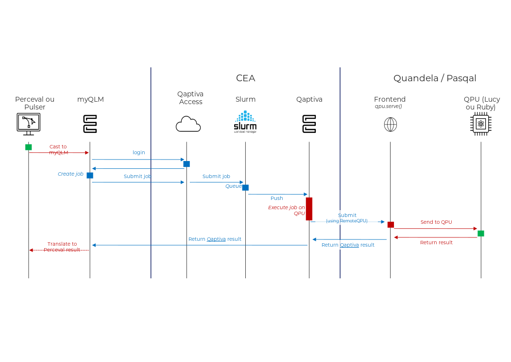
The Qaptiva appliance acts both as a computing ressource and as an intermediate platform to submit jobs to physical QPUs. The figure below shows the typical submission workflow to access a QPU. User agency ends at the myQLM interface.
Qaptiva Hardware
Qaptiva hardware appliance can emulate up to 40 exact qubits. It has an internal queueing system, and all jobs submitted to the appliance will be executed asynchronously. Its hardware specifications are available below:
24 TB of RAM
16 A30 GPU with 24GB of vRAM
384 Intel Cascade Lake 2.4GHz
The same goes for Pulser; Qutip emulation will be used on a compute node but the capabilities of Qaptiva hardware appliance can be used.
Ruby Hardware
Specifications:
Based on Rubidium atoms (monovalent)
Use of Rydberg Blockade for intrication phenomena
Up to 100 atoms
Lucy Hardware
Specifications:
Based on photons and optical circuits
System can be described using Fock States
Up to 12 photons shot in 24 fibers
One environment, different use cases
The quantum software stack provided within ccc-quantum can be used to emulate both digital (gate-based) and analog quantum systems.
By using the free API of myQLM or the default quantum computing libraries provided (Pulser, Perceval), it is possible to emulate locally on a node a quantum system. In this case, it is strongly advised to use a compute node, for a better usage of TGCC computing resources.
By using Qaptiva Access or a dedicated library binding, it is possible to emulate quantum system by harnessing the computing power of the Qaptiva appliance. Qaptiva appliance both offers dedicated hardware with lots of resources (namely, memory) to emulate quantum systems and optimized functions yelding faster computations.
Lastly, Qaptiva Access can also be used to submit jobs on physical QPUs.
Each of these use cases will be discussed in the following sections.
Note
myQLM is an open-source quantum software stack for quantum programs, provided by Eviden.
QLM is the former name of the hardware dedicated to running quantum emulation.
Qaptiva now encompass the hardware and software appliances dedicated to quantum emulation.
Qaptiva Access (also known as QLMaaS) is the interface users can queue quantum jobs with on Qaptiva hardware or on physical QPUs.
Qaptiva-HPC is a standalone software that allows to run myQLM programs on classical compute nodes.
Examples: basic programs
The following examples will show how to use the provided software stack on a compute node.
To launch tutorials provided in /opt/tutorial please refer to the Graphical Environment section.
myQLM
This simple program explores a simple case of digital (gate-based) quantum programming, with the application of multiple Hadamard (H) and CNOT gates using myQLM on a qubit state. The theoretical probability is 0.25 for the state 000, 001, 110 and 111.
from qat.lang.AQASM import Program, H, CNOT

# Create a Program
qprog = Program()
# Number of qubits
nbqubits = 3
# Allocate some qubits
qubits = qprog.qalloc(nbqubits)

# Apply some quantum Gates
qprog.apply(H, qubits[0])
qprog.apply(CNOT, qubits[0], qubits[1])
qprog.apply(CNOT, qubits[1], qubits[2])
qprog.apply(H, qubits[2])
# Export this program into a quantum circuit
circuit = qprog.to_circ()
circuit.display()

# Import one Quantum Processor Unit Factory
from qat.qpus import PyLinalg

# Create a Quantum Processor Unit
qpu = PyLinalg()

# Create job and submit it
job = circuit.to_job(nbshots=10000)
result = qpu.submit(job)

# Print results
for sample in result:
    print("The state {} have a probability measured equal to {}".format(sample.state, sample.probability))
As you can see, increasing the number of shots tends towards the theoretical result.
More example programs are provided in the official QLM documentation. Official tutorials from myQLM are also available directly within ccc-quantum container image at /opt/tutorials/myqlm.
Pulser
This is a simple example of analog computing with Pulser. This example, adapted from the official Pulser documentation, shows how to create an antiferromagnetic state.
import numpy as np
import pulser
import qutip
from pulser_simulation import QutipEmulator

# Setup
L = 8
Omega_max = 2.3 * 2 * np.pi
U = Omega_max / 2.3
delta_0 = -3 * U
delta_f = 1 * U
t_rise = 2000
t_fall = 2000
t_sweep = (delta_f - delta_0) / (2 * np.pi * 10) * 5000

# Define a register: a ring of atoms distanced by a blockade radius distance:
R_inter = pulser.MockDevice.rydberg_blockade_radius(U)
coords = (R_interatomic / (2 * np.tan(np.pi / L))
       * np.array([
         (np.cos(theta * 2 * np.pi / L), np.sin(theta * 2 * np.pi / L))
         for theta in range(L)]))

reg = pulser.Register.from_coordinates(coords, prefix="atom")
reg.draw(blockade_radius=R_inter, draw_half_radius=True, draw_graph=True)

# Define a pulse sequence
rise = pulser.Pulse.ConstantDetuning(pulser.RampWaveform(t_rise, 0.0, Omega_max), delta_0, 0.0)
sweep = pulser.Pulse.ConstantAmplitude(Omega_max, pulser.RampWaveform(t_sweep, delta_0, delta_f), 0.0)
fall = pulser.Pulse.ConstantDetuning(pulser.RampWaveform(t_fall, Omega_max, 0.0), delta_f, 0.0)

seq = pulser.Sequence(reg, pulser.MockDevice)
seq.declare_channel("ising", "rydberg_global")

seq.add(rise, "ising")
seq.add(sweep, "ising")
seq.add(fall, "ising")
seq.draw()

# Emulate the system locally
sim = QutipEmulator.from_sequence(seq, sampling_rate=0.1)
results = sim.run(progress_bar=True)

# Retrieve the results
n_samples = 1000
counts = results.sample_final_state(n_samples)

large_counts = {k: v for k,v in counts.items() if v > 5}
Examples can be found in the official Pulser documentation. The official tutorials (from the GitHub repository) are also available at /opt/tutorials/pulser/.
Perceval
This is a simple example of analog computing with Perceval. This example show how to create a two-mode photonic circuit with one photon injected into each input mode.
import perceval as pcvl
from perceval.algorithm import Sampler
from pprint import pprint

input_state = pcvl.BasicState("|1,1>")
print(f"Input state:", input_state)
circuit = pcvl.BS()
print("Circuit:")
pcvl.pdisplay(circuit)

noise_model = pcvl.NoiseModel(transmittance=0.02, indistinguishability=0.87, g2=0.03)
print(f"Noise model:", noise_model)
experiment = pcvl.Experiment(m_circuit=circuit, noise=noise_model)
print(f"Experiment:")
pcvl.pdisplay(experiment)

processor = pcvl.Processor("SLOS", experiment) # Strong Linear Optical Simulation processor
processor.with_input(input_state)              # Interpreting sampled counts and probabilities

nsamples = 1000  # Number of samples to generate
sampler = Sampler(processor)
# Keep only events where at least two photons are detected.
# This removes outcomes affected by photon loss.
processor.min_detected_photons_filter(2)
samples = sampler.sample_count(nsamples)['results']
print(f"Samples: {samples}")

probs = sampler.probs()['results']
print(f"Probabilities: {probs}")
Examples can be found in the official Perceval documentation. The official tutorials (from the GitHub repository) are also available at /opt/tutorials/perceval/.
Using Qaptiva
From compute nodes to Qaptiva
Using myQLM you can access libraries and tools dedicated to quantum programming. These programs will use pyLinalg as the QPU, a Python-based linear algebra library. Jobs can be submitted on any regular compute node.
Using Qaptiva Access, you will be able to use the Qaptiva hardware appliance, which is also a gateway to physical QPUs.
Note
We recommend using myQLM on a compute node to learn about quantum computing. Once you feel confortable with the concepts, Qaptiva allows to emulate more qubits. Then, real simulation can be run using Ruby (Pasqal QPU) or Lucy (Quandela QPU).
Digital quantum computing
To use Qaptiva appliance in the Qaptiva Access mode, you simply have to change the emulated QPU used, from qat.qpus.PyLinalg to qlmaas.qpus.LinAlg. Since jobs are executed asynchronously, their completion has to be checked before actually using the results.
The example provided in myQLM example can be rewritten:
from qat.lang.AQASM import Program, H, CNOT

# Create a Program
qprog = Program()
# Number of qubits
nbqubits = 3
# Allocate some qubits
qubits = qprog.qalloc(nbqubits)

# Apply some quantum Gates
qprog.apply(H, qubits[0])
qprog.apply(CNOT, qubits[0], qubits[1])
qprog.apply(CNOT, qubits[1], qubits[2])
qprog.apply(H, qubits[2])
# Export this program into a quantum circuit
circuit = qprog.to_circ()
circuit.display()

# Import one Quantum Processor Unit Factory
from qlmaas.qpus import LinAlg

# Create a Quantum Processor Unit
qpu = LinAlg()

# Create job and submit it
job = circuit.to_job(nbshots=10000)
asynchronous_result = qpu.submit(job)

# Wait for the job to complete
result = asynchronous_result.join()

# Print results
for sample in result:
    print("The state {} have a probability measured equal to {}".format(sample.state, sample.probability))
Using GPUs
As Qaptiva appliance comes with GPUs, it is possible to use this units to accelerate the emulation. the qlmaas.qpus.LinAlg constructor takes an argument use_GPU that can be set to True to be executed on GPU. The default is False.
More details can be found in the dedicated documentation on GPU acceleration feature in QLM.
Using Qaptiva-HPC
Introduction
The Qaptiva-HPC QPU emulation engine is very similar to the one running on the Qaptiva appliance, except that it runs directly on the supercomputer nodes without consuming Qaptiva appliance resources.
Qaptiva-HPC allows codes that run on the Qaptiva appliance and utilize the LinAlg, Noisy, and MPSTraj simulated QPUs to be executed on the Irène supercomputer.
Porting myQLM or QaaS code to Qaptiva-HPC
Adapting a code to use Qaptiva-HPC is straightforward. You simply need to replace the QPUs with their Qaptiva-HPC equivalents, according to the following mapping:
QPU on Qaptiva Appliance |
QPU in myQLM |
QPU in Qaptiva-HPC |
|
|
|
|
|
|
|
|
|
As an example, let’s take the following code, which creates a simple Bell pair:
#!/usr/bin/env python
from qat.lang.AQASM import *
from qlmaas.qpus import LinAlg

prog = Program()
qbits = prog.qalloc(2)

prog.apply(H, qbits[0])
prog.apply(CNOT, qbits[0], qbits[1])

circuit = prog.to_circ()
job = circuit.to_job()

linalgqpu = LinAlg()

result = linalgqpu.submit(job)

for sample in result:
    print("State", sample.state, "with amplitude",
        sample.amplitude, "and probability",
        round(sample.probability*100, 2), "%")
You only need to modify the lines highlighted below to obtain the following version:
#!/usr/bin/env python

from qat.lang.AQASM import *
# Modified import
from qat.qpus import DLinAlg

prog = Program()
qbits = prog.qalloc(2)

prog.apply(H, qbits[0])
prog.apply(CNOT, qbits[0], qbits[1])

circuit = prog.to_circ()
job = circuit.to_job()

# Using the distributed QPU
linalgqpu = DLinAlg()
result = linalgqpu.submit(job)

for sample in result:
    print("State", sample.state, "with amplitude",
        sample.amplitude, "and probability",
        round(sample.probability*100, 2), "%")
The process is no more complex than porting a myQLM code to QaaS.
Running code via Command Line
You must load the qaptiva-hpc module to set up the appropriate environment. This is done using the module load qaptiva-hpc command:
$ module load qaptivahpc**
load module cuda/12.9
load module flavor/buildcompiler/gcc/11
load module flavor/gnu/standard
load module c++/gnu/11.2.0
load module c/gnu/11.2.0
load module fortran/gnu/11.2.0
load module gnu/11.2.0
load module flavor/buildmpi/openmpi/4
load module feature/openmpi/mpi_compiler/gcc
load module feature/mkl/single_node
load module feature/openmpi/io/standard
load module feature/openmpi/net/auto
load module flavor/ucx/cuda-12.2
load module flavor/hwloc/standard
load module flavor/libccc_user/hwloc2
load module hwloc/2.9.2
load module pmix/4.2.2
load module feature/hcoll/multicast/enable
load module hcoll/4.8.3221
load module ucx/1.18.1
load module mpi/openmpi/4.1.5
load module python3/3.12
load module qaptivahpc/0.4.0-4
Then, running the code via the command line is similar to myQLM or QaaS. Consider the epr-qaptivahpc.py code listed above:
$ python3 ./epr-qaptiva.py
State |00> with amplitude (0.7071067811865475+0j) and probability 50.0 %
State |11> with amplitude (0.7071067811865475+0j) and probability 50.0 %
Multi-node execution and Batch submission
If the previous execution is performed within a ccc_mprun call, Qaptiva-HPC will automatically implement MPI and deploy across all available nodes, enabling very large-scale simulations.
Here is an example with a code simulating a GHZ state on a number of qubits passed as an argument. For batch execution via the ccc_msub command, use a wrapper script like this:
#!/bin/bash
#### Metadata
#MSUB -r "Qaptiva-HPC"
#MSUB -c 80
#MSUB -n 32
#MSUB -T 18000
#MSUB -q rome
#MSUB -m scratch,work

module purge
module load qaptivahpc
ccc_mprun python3 ./GHZ_param_qhpc.py 36
The number of cores (and nodes) required doubles every time an additional qubit is added to the simulation:
Number of Nodes |
Number of Qubits |
|---|---|
|
|
|
|
|
|
|
|
|
|
|
|
|
|
Using Ruby
Running a Pulser job on Qaptiva
It is possible to emulate quantum system designed with Pulser on Qaptiva. To do so, you need to use:
AnalogQPU from myQLM, that allows to emulate an analog QPUs
IsingAQPU from Pulser-myQLM binding, that translates a Pulser quantum system to an object that can be used by Qaptiva.
The quantum system will then be executed on Qaptiva and the result will be a myQLM object.
The last part of the example provided in Pulser example can be rewritten as follows:
from pulser_myqlm import IsingAQPU
from qlmaas.qpus import AnalogQPU

# Create an analog QPU, convert the sequence to a Qaptiva job and run
aqpu = AnalogQPU(n_step=1000)
qpu = IsingAQPU.from_sequence(seq, qpu=aqpu)
job = IsingAQPU.convert_sequence_to_job(seq, nbshots=0)
res = qpu.submit(job)

# Retrieve the results
dict_res = {sample.state: sample.probability for sample in res if sample.probability > 0005}
More examples can be found in the official tutorials (from the GitHub repository), also available at /opt/tutorials/pulser-myqlm/.
Running a job on Ruby
Once your execution has been verified via local classical simulation, you can run it on a physical QPU.
Note
Jobs on the Ruby QPU can only be dispatched via the myQLM interface after logging into the Irene supercomputer.
To access the Pasqal QPU you simply have to change the QPU used to qlmaas.qpus.PasqalQPU. Since jobs are executed asynchronously, their completion has to be checked before actually using the results.
The example provided in Pulser example can be modified to run on Ruby:
import pulser_myqlm
import qlmaas.qpus

qpu = qlmaas.qpus.PasqalQPU()
job = pulser_myqlm.IsingAQPU.convert_sequence_to_job(seq, nbshots=nbshots, modulation=modulation)
res = qpu.submit(job)
Using Lucy
Quandela provides a learning platform to use their tools: Quandela Training Center.
From Qaptiva simulation to Lucy
Once your Perceval script execution has been verified via local classical simulation, you can run it on a physical QPU.
Note
Jobs on the Lucy QPU can only be dispatched via the myQLM interface after logging into the Irene supercomputer.
Physical properties of the Lucy QPU can be retrieved using the command below:
from qlmaas.qpus import QuandelaQPU
from perceval_interop import MyQLMHelper

qpu_access = QuandelaQPU()

probs = sampler.probs()['results']
print(f"Probabilities: {probs}")
hardware_specs = qpu_access.get_specs()
performances = MyQLMHelper.retrieve_perf(hardware_specs)

print(f"- Indistinguishability (HOM) = {performances['HOM (%)']}%")
print(f"- Transmittance              = {performances['Transmittance (%)']}%")
print(f"- Purity (g2)                = {performances['g2 (%)']}%")

constraints = MyQLMHelper.retrieve_specs(hardware_specs)['constraints']

print(f"- Mode counts   = [{constraints['min_mode_count']}-{constraints['max_mode_count']}]")
print(f"- Photon counts = [{constraints['min_photon_count']}-{constraints['max_photon_count']}]")
The machine’s average performance metrics are:
Indistinguishability: 90%
Transmittance: 2%
Purity: 2%
These metrics are indicative and are subject to change.
Running a job on Lucy
To access the Quandela QPU you simply have to change the QPU used to qlmaas.qpus.QuandelaQPU. Since jobs are executed asynchronously, their completion has to be checked before actually using the results.
The example provided in Perceval example can be rewritten:
import perceval as pcvl

from qlmaas.qpus import QuandelaQPU
from perceval_interop import MyQLMHelper

input_state = pcvl.BasicState("|1,1>")
circuit = pcvl.BS()

qpu_access = QuandelaQPU()

experiment = pcvl.Experiment(m_circuit=circuit)
experiment.with_input(input_state)
experiment.min_detected_photons_filter(1)

print("Experiment:")
pcvl.pdisplay(experiment)

nb_samples = 1000
max_shots = 1000 * nb_samples

job = MyQLMHelper.make_job(
    "sample_count", experiment, max_shots=max_shots, max_samples=nb_samples
)

qpu_access = QuandelaQPU()
results = qpu_access.submit(job)

nb_samples = 1000
max_shots = 1000 * nb_samples

job = MyQLMHelper.make_job(
    "sample_count", experiment, max_shots=max_shots, max_samples=nb_samples
)

qpu_access = QuandelaQPU()
results = qpu_access.submit(job)
Using MerLin on Lucy
MerLin enables researchers to build, train, and benchmark photonic quantum machine learning models using familiar ML tools.
Built upon PyTorch, it allows hybrid quantum-classical models within standard machine learning workflow.
More details are provided in the official MerLin documentation.
Basic Usage: Simple Quantum Layer
This minimal example exposes the initilization and training of a single quantum layer.
Here, the model learns to distinguish the two concentric-circle classes from their 2D coordinates.
import torch
import numpy as np
import merlin as ML
from sklearn.datasets import make_circles
from sklearn.model_selection import train_test_split

# Dataset
X, y = make_circles(n_samples=400)
X_train, X_test, y_train, y_test = train_test_split(X, y, test_size=0.2, random_state=42)

# Normalize using training data statistics (prevent data leakage)
min_vals = X_train.min(axis=0, keepdims=True)
max_vals = X_train.max(axis=0, keepdims=True)
X_train = (X_train - min_vals) / np.clip(max_vals - min_vals, a_min=1e-6, a_max=None)
X_test = (X_test - min_vals) / np.clip(max_vals - min_vals, a_min=1e-6, a_max=None)

X_train = torch.tensor(X_train, dtype=torch.float32)
y_train = torch.tensor(y_train, dtype=torch.long)

# Quantum layer
quantum_layer = ML.QuantumLayer.simple(
    input_size=2,
    output_size=2,
)

# Training loop
optimizer = torch.optim.Adam(quantum_layer.parameters(), lr=0.01)
criterion = torch.nn.CrossEntropyLoss()

for _ in range(100):
    optimizer.zero_grad()
    logits = quantum_layer(X_train)
    loss = criterion(logits, y_train)
    loss.backward()
    optimizer.step()

X_test = torch.tensor(X_test, dtype=torch.float32)
y_test = torch.tensor(y_test, dtype=torch.long

with torch.no_grad():
    test_logits = quantum_layer(X_test)
    predictions = test_logits.argmax(dim=1)
    correct = (predictions == y_test).sum().item()
    accuracy = correct / y_test.size(0)

print(f"correct: {correct}")
print(f"accuracy: {accuracy:.3f}")
Advanced Usage: Hybrid Quantum-Classical Model
This example shows how to initilize, train and infer an hybrid model based on classical PyTorch Layer and the MerLin Quantum Layer.
It also shows how to execute the model on the remote quantum processor.
import torch
import torch.nn as nn
import merlin as ML
from merlin.datasets import iris

train_features, train_labels, _ = iris.get_data_train()
test_features, test_labels, _ = iris.get_data_test()

# Convert data to PyTorch tensors
X_train = torch.FloatTensor(train_features)
y_train = torch.LongTensor(train_labels)
X_test = torch.FloatTensor(test_features)
y_test = torch.LongTensor(test_labels)
X_lucy = X_test[:30]
y_lucy = y_test[:30]

class HybridIrisClassifier(nn.Module):
    def __init__(self):
        super().__init__()

        # Classical preprocessing layer: 4 -> 8 -> 3
        self.classical_in = nn.Sequential(
            nn.Linear(4, 8),
            nn.ReLU(),
            nn.Linear(8, 3),
            nn.Tanh(),  # Normalize to [-1, 1] for quantum layer
        )

        # Quantum hidden layer:  3 -> quantum
        self.quantum = ML.QuantumLayer.simple(input_size=3)

        # Classical output layer: quantum -> 8 -> 3
        self.classical_out = nn.Sequential(
            nn.Linear(self.quantum.output_size, 8),
            nn.ReLU(),
            nn.Linear(8, 3),
        )

    def forward(self, x):
        x = self.classical_in(x)
        x = (x + 1) / 2
        x = self.quantum(x)
        return self.classical_out(x)

# Classical training parameters
learning_rate = 0.0045
number_of_epochs = 300

# Lucy sampling parameters
lucy_nsample = 1000
lucy_microbatch_size = 8

# Training function as you would use it in a classical PyTorch pipeline
def train_hybrid_model(seed=123, epochs=number_of_epochs, lr=learning_rate):
    torch.manual_seed(seed)
    trained_model = HybridIrisClassifier()
    optimizer = torch.optim.Adam(trained_model.parameters(), lr=lr)
    criterion = nn.CrossEntropyLoss()

    for epoch in range(1, epochs + 1):
        trained_model.train()
        optimizer.zero_grad()
        outputs = trained_model(X_train)
        loss = criterion(outputs, y_train)
        loss.backward()
        optimizer.step()

    trained_model.eval()
    return trained_model

# Train the model
model = train_hybrid_model()

lucy_predictions, lucy_accuracy = None, None

try:
    from perceval_interop import MyQLMSession
    from qlmaas.qpus import QuandelaQPU

    # We allocate a session on Lucy as we need a QPU for the inference
    session = MyQLMSession(QuandelaQPU())
    # The remote processor uses that session to process data
    merlin_processor = ML.MerlinProcessor(
        session=session,
        microbatch_size=lucy_microbatch_size,
        timeout=7200.0,
        max_shots_per_call=lucy_nsample * lucy_microbatch_size,
    )

    model.eval()
    with torch.no_grad():
        # We can then use the remote processor to execute the trained model
        lucy_outputs = merlin_processor.forward(
            model,
            X_lucy,
            nsample=lucy_nsample,
        )
        lucy_predictions = lucy_outputs.argmax(dim=1)

    lucy_accuracy = (lucy_predictions == y_lucy).float().mean().item()
    print(f"Lucy accuracy on {X_lucy.shape[0]} samples: {lucy_accuracy:.4f}")
except Exception as error:
    print("Lucy evaluation could not be completed.")
    print(f"Reason: {error}")