Process distribution, affinity and binding
Hardware topology
Hardware topology is the organization of cores, processors, sockets, memory, network cards and accelerators (like graphic cards) in a node. An image of the topology of a node is shown by lstopo. This function comes with hwloc, and you can access it with the command module load hwloc. For example, a simple graphical representation of a compute node layout can be obtained with:
lstopo --no-caches --no-io --of png
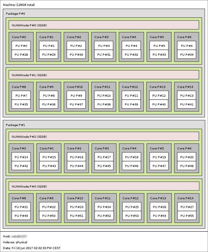
Hardware topology of a 28 core node with 4 sockets and SMT (Simultaneous Multithreading, as Hyper-threading on Intel architecture)
Definitions
We define here some vocabulary:
- Process distribution : the distribution of MPI processes describes how these processes are spread across the cores, sockets or nodes.
- Process affinity : represents the policy of resources management (cores and memory) for processes.
- Process binding : a Linux process can be bound (or stuck or pinned) to one or many cores. It means a process and its threads can run only on a given selection of cores.
The default behavior for distribution, affinity and binding is managed by the batch scheduler through the ccc_mprun command. SLURM is the batch scheduler for jobs on the supercomputer. SLURM manages the distribution, affinity and binding of processes even for sequential jobs. That is why we recommend you to use ccc_mprun even for non-MPI codes.
Process distribution
We present here the most common MPI process distributions. The cluster naturally has a two dimensional distribution. The first level of distribution manages the process layout across nodes and the second level manages process layout within a node, across sockets.
- Distribution across nodes
- block by node: The block distribution method will distribute tasks such that consecutive tasks share a node.
- cyclic by node: The cyclic distribution method will distribute tasks such that consecutive tasks are distributed over consecutive nodes (in a round-robin fashion).
- Distribution across sockets
- block by socket: The block distribution method will distribute tasks to a socket such that consecutive tasks share a same socket.
- cyclic by socket: The cyclic distribution method will distribute tasks to a socket such that consecutive tasks are distributed over consecutive socket (in a round-robin fashion).
The default distribution on the supercomputer is block by node and block by socket. To change the distribution of processes, you can use the option -E "-m block|cyclic:[block|cyclic]" for ccc_mprun or for ccc_msub. The first argument refers to the node level distribution and the second argument refers to the socket level distribution.
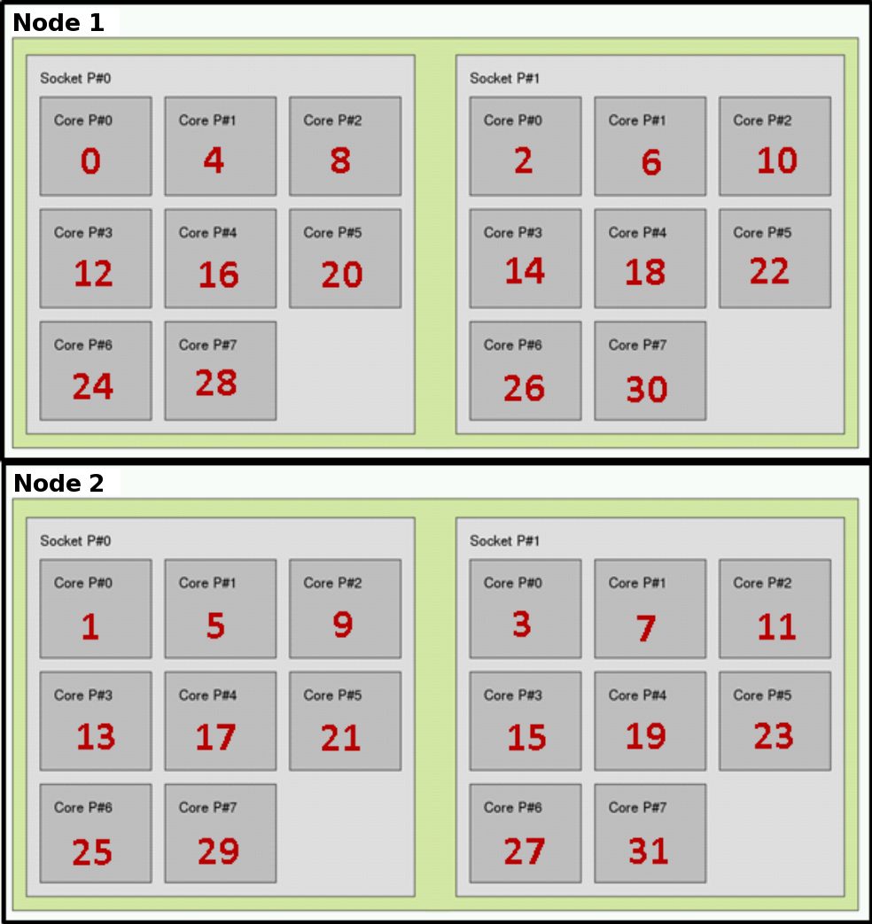
In the following examples, let us consider 2 nodes composed of 2 sockets. Each socket with 8 cores.
Block by node and block by socket distribution:
ccc_mprun -n 32 -E '-m block:block' -A <project> ./a.out
- Processes 0 to 7 are gathered on the first socket of the first node
- Processes 8 to 15 are gathered on the second socket of the first node
- Processes 16 to 23 are gathered on the first socket of the second node
- Processes 24 to 31 are gathered on the second socket of the second node
This is the default distribution.
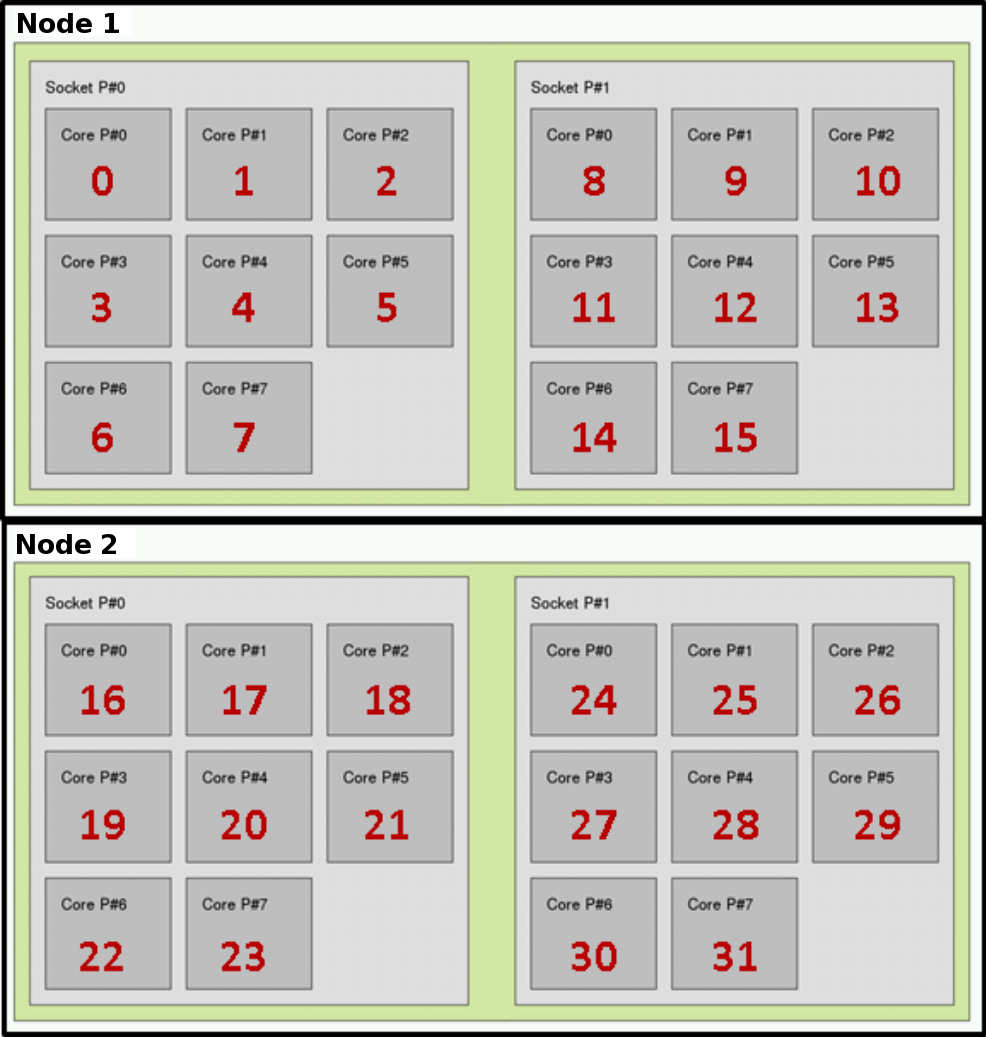
Cyclic by node and block by socket distribution:
ccc_mprun -n 32 -E '-m cyclic:block' -A <project> ./a.out
- Process 0 runs on the first socket of the first node
- Process 1 runs on the first socket of the second node
- …
And once the first socket is full, processes are distributed on the next sockets:
- Process 16 runs on the second socket of the first node
- Process 17 runs on the second socket of the second node
- …
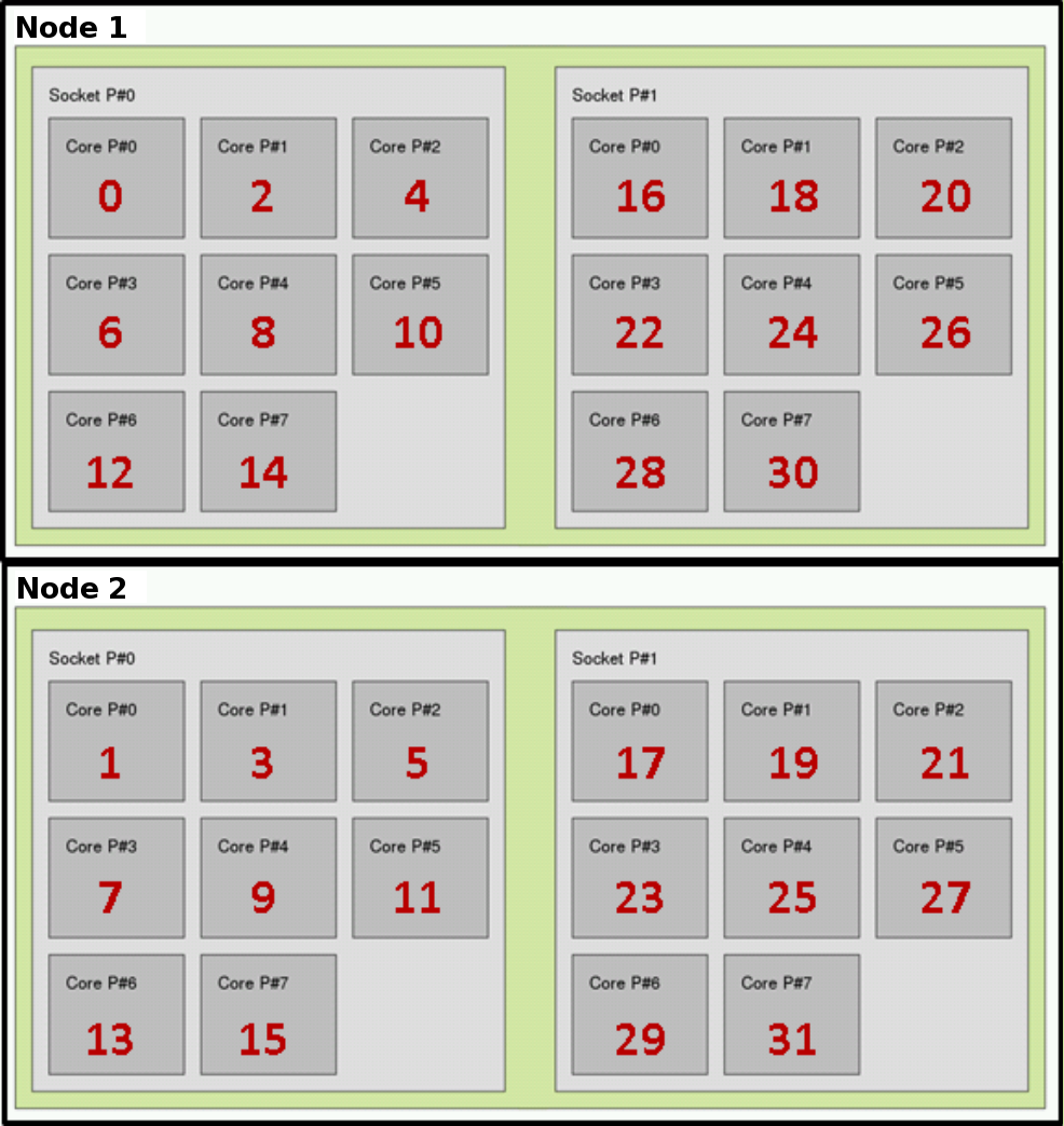
Block by node and cyclic by socket distribution:
ccc_mprun -n 32 -E '-m block:cyclic' ./a.out
- Process 0 runs on the first socket of the first node
- Process 1 runs on the second socket of the first node
- …
And once the first node is full, processes are distributed on both sockets of the next node:
- Process 16 runs on the first socket of the second node
- Process 17 runs on the second socket of the second node
- …
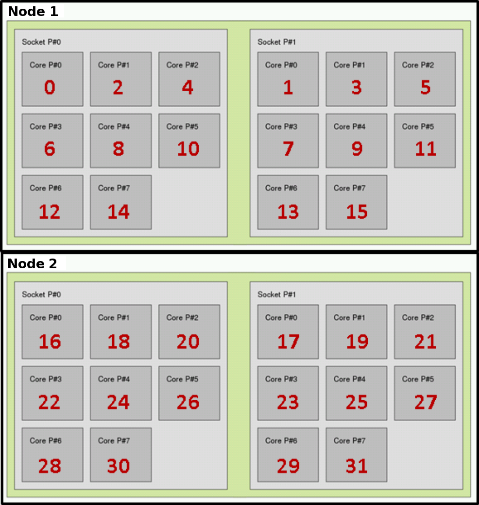
Cyclic by node and cyclic by socket distribution:
ccc_mprun -n 32 -E '-m cyclic:cyclic' <project> ./a.out
- Process 0 runs on the first socket of the first node
- Process 1 runs on the first socket of the second node
- Process 2 runs on the second socket of the first node
- Process 3 runs on the second socket of the second node
- Process 4 runs on the first socket of the first node
- …
Process and thread affinity
Why is affinity important for improving performance ?
Most recent nodes are NUMA nodes: they need more time to access some regions of memory than others, because all memory regions are not physically on the same bus.
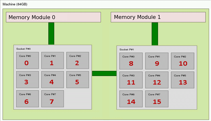
NUMA node : Memory access
This picture shows that if a data is in the memory module 0, a process running on the second socket like the 9th process will take more time to access the data. We can introduce the notion of local data vs remote data. In our example, if we consider a process running on the socket 0, a data is local if it is on the memory module 0. The data is remote if it is on the memory module 1.
We can then deduce the reasons why tuning the process affinity is important:
- Data locality improve performance. If your code uses shared memory (like pthreads or OpenMP), the best choice is to group your threads on the same socket. The shared data should be local to the socket and moreover, the data may stay in the processor’s cache.
- System processes can interrupt your process running on a core. If your process is not bound to a core or to a socket, it can be moved to another core or to another socket. In this case, all data for this process have to be moved with the process too and it can take some time.
- MPI communications are faster between processes which are on the same socket. If you know that two processes have many communications, you can bind them to the same socket.
- On Hybrid nodes, the GPUs are connected to buses which are local to a socket. Processes can take more time to access a GPU which is not connected to its socket.
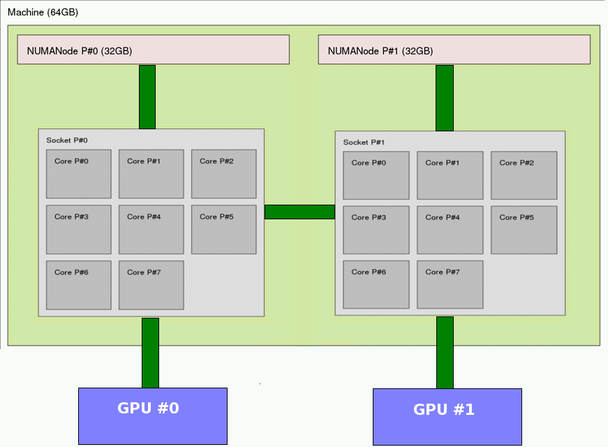
NUMA node : Example of a hybrid node with GPU
For all these reasons, knowing the NUMA configuration of the partition’s nodes is strongly recommended. The next section presents some ways to tune your processes affinity for your jobs.
Process/thread affinity
The batch scheduler sets a default binding for processes. Each process is bound to the core it was distributed to, as described in Process distribution.
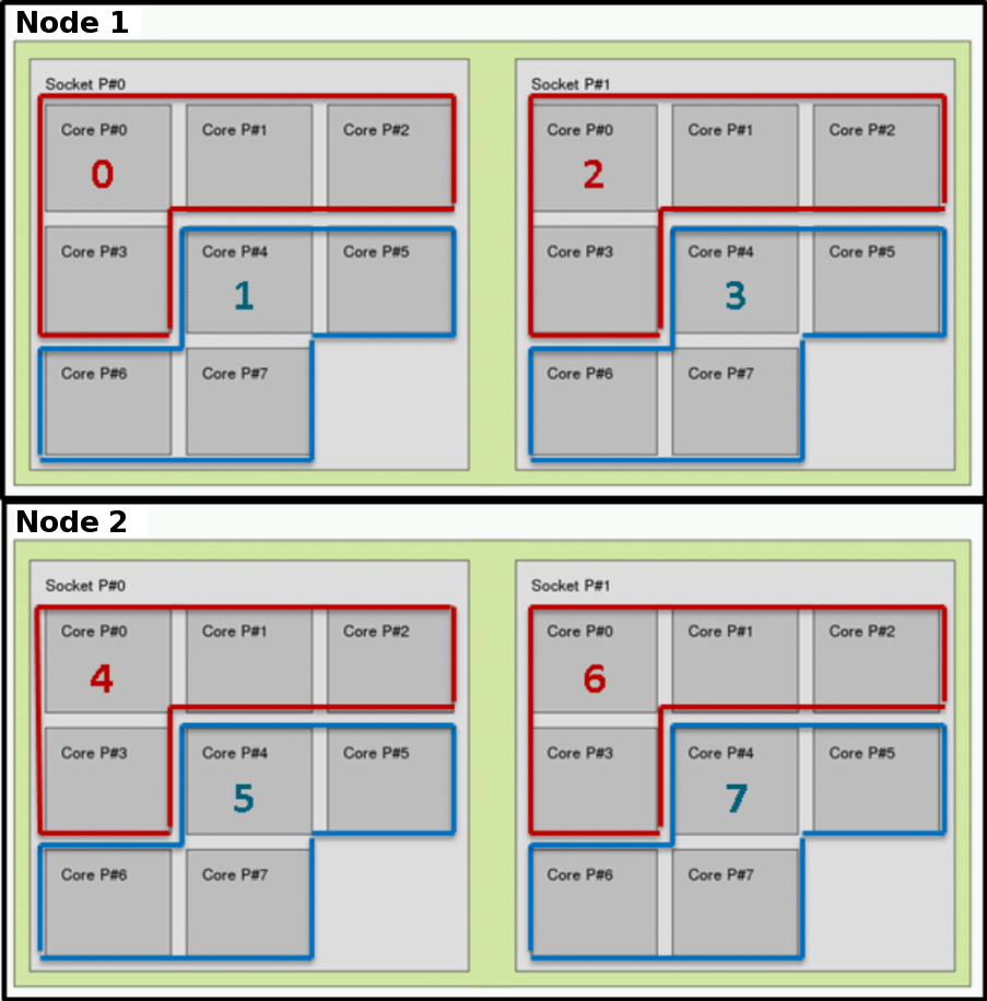
For multi-threaded jobs, the batch scheduler provides the option -c to bind each process to several cores. Each thread created by a process will inherit its affinity. Here is an example of a hybrid OpenMP/MPI code running on 8 MPI processes, each process using 4 OpenMP threads.
#!/bin/bash
#MSUB -r MyJob_Para                # Job name
#MSUB -n 8                         # Number of tasks to use
#MSUB -c 4                         # Assign 4 cores per process
#MSUB -T 1800                      # Elapsed time limit in seconds
#MSUB -o example_%I.o              # Standard output. %I is the job id
#MSUB -A <project>                 # Project ID
#MSUB -q <partition>               # Partition

export OMP_NUM_THREADS=4
ccc_mprun ./a.out
The process distribution will take the -c option into account and set the binding accordingly. For example, in the default block:block mode:
- Process 0 is bound to cores 0 to 3 of the first node
- Process 1 is bound to cores 4 to 7 of the first node
- Process 2 is bound to cores 8 to 11 of the first node
- Process 3 is bound to cores 12 to 15 of the first node
- Process 4 is bound to cores 0 to 3 of the second node
- …
Note
Since the default distribution is block, with the -c option, the batch scheduler will try to gather the cores as close as possible. This usually provides the best performances for multi-threaded jobs. In the previous example, all the cores of a MPI process will be located on the same socket.
Thread affinity may be set even more thoroughly within the process binding. For example, check out the Intel thread affinity description.
Hyper-Threading usage
SMT (Simultatneous Multithreading, as Hyper-threading on Intel architecture) and its implementations are used to improve parallelization of computations. It is activated on compute nodes. Therefore, each physical core appears as two processors to the operating system, allowing concurrent scheduling of two processes or threads per core. Unless specified, the resource manager will only consider physical cores and ignore this feature.
In case an application may positively benefits from this technology, MPI processes or OpenMP threads can be bind to logical cores. Here is the procedure:
- Doubling the processes:
#!/bin/bash
#MSUB -q <partition>
#MSUB -n 2
#MSUB -A <projet>

ccc_mprun -n $((BRIDGE_MSUB_NPROC*2)) -E'--cpu_bind=threads --overcommit' ./a.out   # 4 processes are run on 2 physical cores
- Doubling the threads:
#!/bin/bash
#MSUB -q <partition>
#MSUB -n 2
#MSUB -c 8
#MSUB -A <project>

export OMP_NUM_THREADS=$((BRIDGE_MSUB_NCORE*2))   # threads number must be equal to logical cores
ccc_mprun ./a.out   # each process runs 16 threads on 8 physical cores / 16 logical cores
Turbo
The processor turbo technology (Intel Turbo Boost or AMD turbo core) is available and activated by default on Irene. This technology dynamically adjusts CPU frequency in order to reach the highest frequency allowed by the available power and thermal limits. The Turbo can be responsible of performance variation because of hardware differences between two nodes and if other jobs are running on the same node. One can choose to disable this technology by loading the module feature/system/turbo_off:
module load feature/system/turbo_off
Deactivating this technology allows a better control of the timing of the execution of the codes but can trigger poor performances. One can choose to have capped performances by loading the feature feature/system/turbo_capped:
module load feature/system/turbo_capped
which sets the CPU frequency to a determined value which prevents Turbo to be activated for vectorized operations.